Fitting a Lens image using Levenberg-Marquardt#
In this hypothetical scenario we have an image of galaxy galaxy strong lensing and we would like to recover a model of this scene. Thus we will need to determine parameters for the background source light, the lensing galaxy light, and the lensing galaxy mass distribution. In this notebook we will assume the user has some method to find approximate parameters for all the models (perhaps guess and check by eye, a neural network, or a random number generator and a lot of computing power), once we are close to the optimal solution, Levenberg Maquardt can quickly converge to it. Note that LM will converge to a local minimum, so we need to make sure it’s the right local minimum by giving it a good start!
import caustics
import numpy as np
import torch
import matplotlib.pyplot as plt
from matplotlib.patches import Ellipse
from scipy.stats import norm
Specs for the data#
These are some properties of the data that aren’t very interesting for the demo, it includes the size of the image, pixelscale, noise level, etc.
# Data specs

background_rms = 0.005  #  background noise per pixel
exp_time = 1000.0  #  exposure time (arbitrary units, flux per pixel is in units #photons/exp_time unit)
numPix = 60  #  cutout pixel size per axis
pixelscale = 0.05  #  pixel size in arcsec (area per pixel = pixel_scale**2)
fwhm = 0.05  # full width at half maximum of PSF
psf_sigma = fwhm / (2 * np.sqrt(2 * np.log(2)))
psf_type = "GAUSSIAN"  # 'GAUSSIAN', 'PIXEL', 'NONE'

cosmology = caustics.FlatLambdaCDM(name="cosmo")
cosmology.to(dtype=torch.float32)

upsample_factor = 1
quad_level = 3
thx, thy = caustics.utils.meshgrid(
    pixelscale / upsample_factor,
    upsample_factor * numPix,
    dtype=torch.float32,
)
z_l = torch.tensor(0.5, dtype=torch.float32)
z_s = torch.tensor(1.5, dtype=torch.float32)
Build simulator forward model#
Here we build the caustics simulator which will handle the lensing and generating our images for the sake of fitting. It includes a model for the lens mass distribution, lens light, and source light. We also include a simple gaussian PSF for extra realism, though for simplicity we will use the same PSF model for simulating the mock data and fitting.
# Set up the forward model

# Lens mass model (SIE + shear)
lens_sie = caustics.SIE(
    name="galaxylens",
    cosmology=cosmology,
    x0=0.05,
    y0=0.0,
    q=0.86,
    phi=-0.20,
    Rein=0.66,
)
lens_sie.to_dynamic()

lens_shear = caustics.ExternalShear(
    name="externalshear",
    cosmology=cosmology,
    x0=0.0,
    y0=0.0,
    gamma_1=0.0,
    gamma_2=-0.05,
)
lens_shear.gamma_1.to_dynamic()
lens_shear.gamma_2.to_dynamic()

lens_mass_model = caustics.SinglePlane(
    name="lensmass",
    cosmology=cosmology,
    lenses=[lens_sie, lens_shear],
    z_l=z_l,
    z_s=z_s,
)

# Lens light model (sersic)
lens_light_model = caustics.Sersic(
    name="lenslight",
    x0=0.05,
    y0=0.0,
    q=0.75,
    phi=1.18,
    n=2.0,
    Re=0.6 / np.sqrt(0.75),
    Ie=16 * pixelscale**2,
)
lens_light_model.to_dynamic()

# Source light model (sersic)
source_light_model = caustics.Sersic(
    name="sourcelight",
    x0=0.1,
    y0=0.0,
    q=0.75,
    phi=1.18,
    n=1.0,
    Re=0.1 / np.sqrt(0.75),
    Ie=16 * pixelscale**2,
)
source_light_model.to_dynamic()

# Gaussian PSF Model
psf_image = caustics.utils.gaussian(
    nx=upsample_factor * 6 + 1,
    ny=upsample_factor * 6 + 1,
    pixelscale=pixelscale / upsample_factor,
    sigma=psf_sigma,
    upsample=2,
)

# Image plane simulator
sim = caustics.LensSource(
    lens=lens_mass_model,
    lens_light=lens_light_model,
    source=source_light_model,
    psf=psf_image,
    pixels_x=numPix,
    pixelscale=pixelscale,
    upsample_factor=upsample_factor,
    quad_level=quad_level,
)
Sample some mock data#
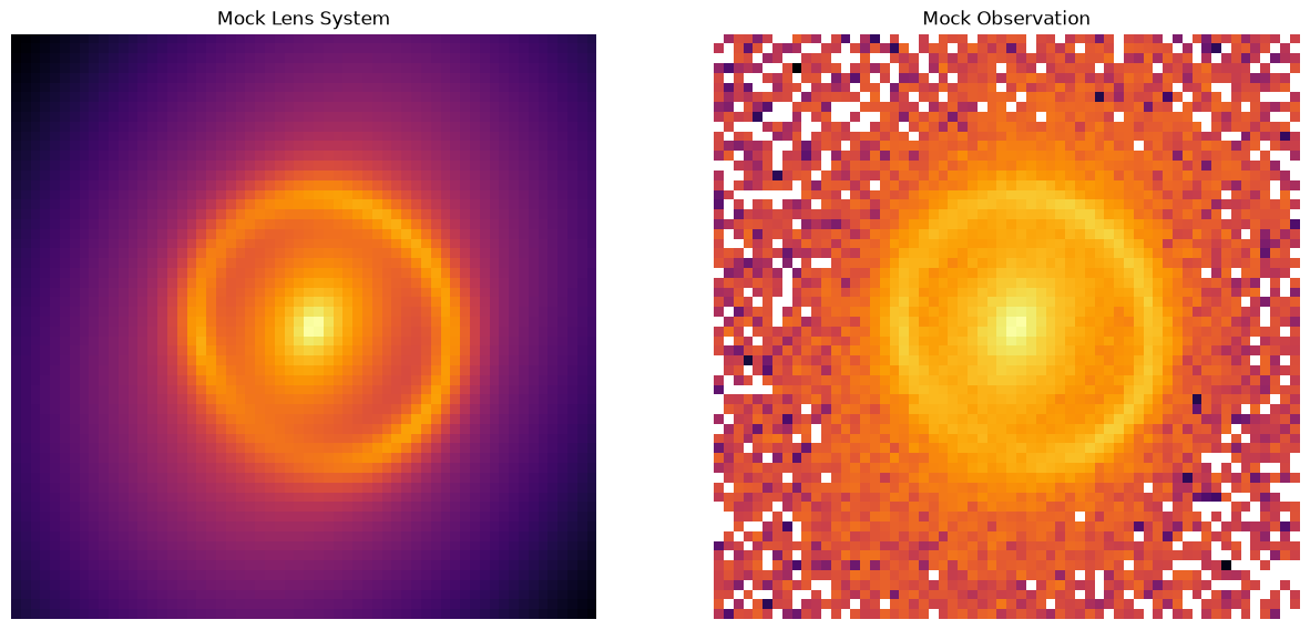
Here we write out the true values for all the parameters in the model. In total there are 21 parameters, so this is quite a complex model already! We then plot the data so we can see what it is we re trying to fit.
tensor([ 0.0500,  0.0000,  0.8600, -0.2000,  0.6600,  0.0000, -0.0500,  0.1000,
         0.0000,  0.7500,  1.1800,  1.0000,  0.1155,  0.0400,  0.0500,  0.0000,
         0.7500,  1.1800,  2.0000,  0.6928,  0.0400], dtype=torch.float64)
1.0084377412630428
/tmp/ipykernel_1125/3132726071.py:26: RuntimeWarning: invalid value encountered in log10
  np.log10(obs_system.detach().cpu().numpy()), cmap="inferno", origin="lower"
Fit using Levenberg-Marquardt#
Since caustics is differentiable, it is very easy to write a Levenberg-Marquardt implementation (second order gradient descent). caustics includes a basic implementation of LM though there are more sophisticated versions out there.
To start we take the true parameters, copy them 10 times, and randomly perturb their values to simulate some process where we find close initial parameters for our model, but we haven’t yet reached the maximum likelihood point. The fit itself only takes a minute to run all 10 starting points. In a real analysis you may be farther from the true parameters at initialization, but you could run hundreds or thoustands of starting points relatively cheaply to find the maximum likelihood.
batch_inits = true_params.clone().repeat((10, 1))
# starting points will not be at true values, so we add noise
batch_inits += 0.01 * torch.randn_like(batch_inits)
batch_inits = batch_inits.to(dtype=torch.float32)
res = caustics.utils.batch_lm(
batch_inits,
obs_system.reshape(-1).repeat(10, 1).to(dtype=torch.float32),
lambda x: sim(x).reshape(-1),
C=variance.reshape(-1).repeat(10, 1),
)
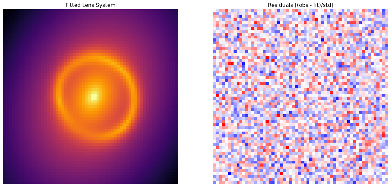
best_fit = res[0][np.argmin(res[2].numpy())]
print(res[2] / np.prod(obs_system.shape))
tensor([1.0017, 1.0017, 1.0017, 1.0017, 1.0017, 1.0017, 1.0017, 1.0017, 1.0017,
        1.0017])
tensor([ 5.2502e-02,  2.8453e-03,  8.5637e-01, -2.5920e-01,  6.5912e-01,
         8.7500e-04, -5.3775e-02,  9.9747e-02,  1.8244e-03,  7.4533e-01,
         1.2123e+00,  1.0193e+00,  1.1459e-01,  3.9695e-02,  5.0504e-02,
         8.5950e-04,  7.3221e-01,  1.1796e+00,  1.9821e+00,  7.0582e-01,
         3.9823e-02]) tensor([ 0.0500,  0.0000,  0.8600, -0.2000,  0.6600,  0.0000, -0.0500,  0.1000,
         0.0000,  0.7500,  1.1800,  1.0000,  0.1155,  0.0400,  0.0500,  0.0000,
         0.7500,  1.1800,  2.0000,  0.6928,  0.0400], dtype=torch.float64)
Examine uncertainties#
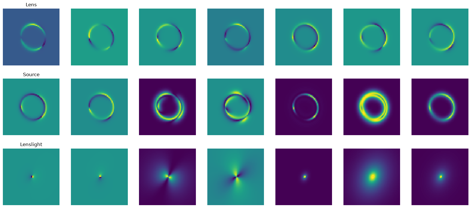
A neat part about having a differentiable model is that we can easily compute derivatives and inspect our models. Below we compute the jacobian, which is a series of images that show how the model would change if we modified any of the parameters.
The top row shows what would happen if the lens parameters were adjusted, the first 5 are SIE parameters and the last two are Shear parameters.
The middle row shows how the image would change if we modified the source parameters, these represent a lensed Sersic profile.
The bottom row shows how the image would change if we modified the lens light parameters, these represent an unlensed Sersic profile.
# Compute jacobian
J = torch.func.jacfwd(lambda x: sim(x))(best_fit)
fig, axarr = plt.subplots(3, 7, figsize=(21, 9))
for i, ax in enumerate(axarr.flatten()):
    ax.imshow(J[..., i], origin="lower")
    if i % 7 == 0:
        ax.set_title(["Lens", "Source", "Lenslight"][i // 7])
    ax.axis("off")
plt.show()
The code cell below uses a covariance matrix to construct a corner plot to display the full uncertainty matrix that we can compute for our model. More is explained below.
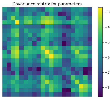
For a \(\chi^2\) optimization problem it is possible to compute a very accurate approximation of the Hessian using just the Jacobian. Since caustics is autodifferentiable we have already easily extracted the Jacobian in a single line, so now we compute the Hessian as: \(H \approx J^T\Sigma^{-1}J\) where \(\Sigma^{-1}\) is the inverse covariance matrix of pixel uncertainties. In our case we know the variance on each pixel so we simply divide by that. Finally the covariance matrix of uncertainties for our model parameters is just the matrix inverse of the Hessian.
J = J.reshape(-1, len(best_fit))
# Compute Hessian
H = J.T @ (J / variance.reshape(-1, 1).to(dtype=torch.float32))
# Compute covariance matrix
C = torch.linalg.inv(H)
plt.imshow(np.log10(np.abs(C.detach().cpu().numpy())))
plt.colorbar()
plt.axis("off")
plt.title("Covariance matrix for parameters")
plt.show()
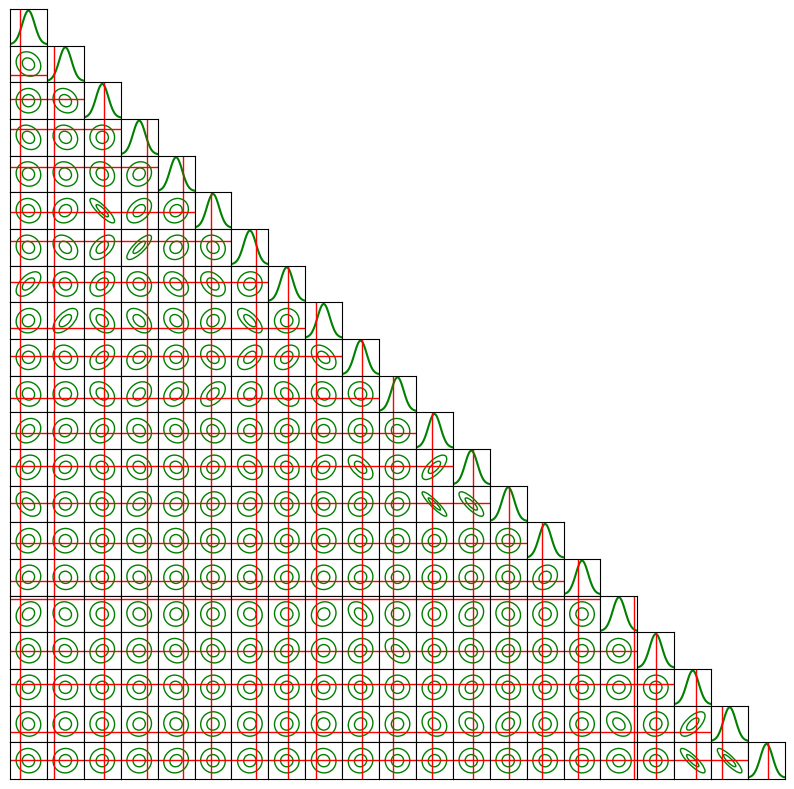
A more helpful visual representation of the uncertainty covariance matrix is the corner plot below. For each parameter on the diagonal, and each pair of parameters on the lower triangle we now see how our fitted values and their uncertainties (green) align with the true parameters (red). As you can see, for the most part, the fitted values plus uncertainty enclose the true parameter. Note that these uncertainties are taken from a taylor expansion at the maximum likelihood and ultimately represent an approximation of the full uncertainty distribution. To fully explore the uncertainties one would need to run an MCMC sampling algorithm which can take a very long time before one will see the non-linear perturbations to the uncertainty in each parameter/pair. We have another notebook which does precisely this for the same mock setup!
corner_plot_covariance(
    C.detach().cpu().numpy(), best_fit.detach().cpu().numpy(), true_values=true_params
)