Caustics with JAX!#
caustics is a powerful gravitational lensing simulator that can support users from beginner to highly advanced. It is also entirely compatible with both PyTorch and JAX. Here we will show a basic example in JAX, but every aspect of caustics that you see in the other tutorials can also be run in JAX.
You may recognize this tutorial as the Caustics Interface: Object Oriented, and you’d be right!
Simulating an SIE lens#
Here we will demo the very basics of lensing with a classic SIE lens model. We will see what it takes to make an SIE model, lens a background Sersic source, and sample the resulting image using a Simulator. caustics simulators can generalize to very complex scenarios, here we will use a built-in simulator which handles a common use case (lensing a background source). To start, we of course need to import some modules. For the minimal example, this is just matplotlib a common package used for plotting, jax which is a numerical package for GPU/autodiff (much like numpy), and caustics the reason you are here.
In this tutorial, we will guide you through the process of simulating an SIE lens using the object-oriented method. This tutorial is mirrored in other tutorials so you can see the yaml, object oriented, and functional interfaces.
First, let’s import the necessary packages:
Import the Necessary Packages#
Note: These packages need to be imported for any method
JAX note you need to tell caustics to run everything in JAX, the easiest way is to set the environment variable CASKADE_BACKEND="jax" since caskade is the simulator backend for caustics.
import os

os.environ["CASKADE_BACKEND"] = "jax"

import matplotlib.pyplot as plt
import jax.numpy as jnp
import jax
import caustics
JAX note It is also possible to set the backend after importing caustics. But this is dangerous in case some PyTorch tensors have already been created.
# caustics.backend.backend = "jax"
Define a Cosmology#
Before we can begin gravitational lensing, we need to know what kind of universe we are in. This is used for calculating various distances and timescales (depending on the problem) since gravitational lensing typically occurs over cosmologically significant distances in the universe. Here we define a standard flat Lambda Cold Dark Matter cosmology. Nothing fancy here, but it’s still needed.
cosmology = caustics.FlatLambdaCDM()
Lens Mass Distribution#
In order for gravitational lensing to occur, we need some mass to bend the light. Here we define a basic Singular Isothermal Ellipsoid (SIE), which is a versatile profile used in many strong gravitational lensing simulations. As the first argument, we pass the cosmology so that the SIE can compute various quantities which make use of redshift information (seen later). Each model must have a unique name so we call this one lens though you can also let caustics automatically pick a unique name.
sie = caustics.SIE(
    cosmology=cosmology,
    name="lens",
    z_l=0.5,
    z_s=1.5,
    x0=-0.2,
    y0=0.0,
    q=0.4,
    phi=1.5708,
    Rein=1.7,
)
sie.to_dynamic()
Source Light Distribution#
If we wish to see anything in our lensing configuration then we need a bright object in the background to produce some light that will pass through (and be bent by) our lens mass distribution. Here we create a Sersic light model which is a common versatile profile for representing galaxies. Note that we don’t need to pass a light model any Cosmology information, since light models essentially just define a function on (x,y) coordinates that gives a brightness, the lens models handle all cosmology related calculations. For the name we very creatively choose source.
src = caustics.Sersic(
    name="source", x0=0.0, y0=0.0, q=0.5, phi=-0.985, n=1.3, Re=1.0, Ie=5.0
)
src.to_dynamic()
Sersic Lens Light Distribution#
The source isn’t the only bright thing in the sky! The lensing galaxy itself will also have bright stars and can be seen as well. Let’s add another Sersic model with the name lenslight.
lnslt = caustics.Sersic(
    name="lenslight", x0=-0.2, y0=0.0, q=0.8, phi=0.0, n=1.0, Re=1.0, Ie=10.0
)
lnslt.to_dynamic()
Lens Source Simulator#
Next we pass our configuration to a Simulator in caustics, simulators perform the work of forward modelling various configurations and producing the desired outputs. Here we are interested in a common scenario of producing an image of a background source through a lens distribution. It is possible to make your own simulator to represent all sorts of situations. First, we pass the lens model and the source model defined above. Next we use pixelscale and pixels_x to define the grid of pixels that will be sampled. Finally, we pass the z_s redshift at which the source (Sersic) model should be placed; recall that light models don’t use the cosmology model and so aren’t aware of their placement in space.
sim = caustics.LensSource(
    lens=sie, source=src, lens_light=lnslt, pixelscale=0.05, pixels_x=100, quad_level=3
)
# Print out the order of model parameters
# Note that parameters with values are "static" so they don't need to be provided by you
print(sim)
sim|LensSource
    psf|static: 1
    x0|static: 0
    y0|static: 0
    lens|SIE
        FlatLambdaCDM|FlatLambdaCDM
            h0|static: 0.677
            critical_density_0|static: 1.27e+11
            Om0|static: 0.31
        z_s|dynamic: 1.5
        z_l|dynamic: 0.5
        x0|dynamic: -0.2
        y0|dynamic: 0
        q|dynamic: 0.4
        phi|dynamic: 1.57
        Rein|dynamic: 1.7
    source|Sersic
        x0|dynamic: 0
        y0|dynamic: 0
        q|dynamic: 0.5
        phi|dynamic: -0.985
        n|dynamic: 1.3
        Re|dynamic: 1
        Ie|dynamic: 5
    lenslight|Sersic
        x0|dynamic: -0.2
        y0|dynamic: 0
        q|dynamic: 0.8
        phi|dynamic: 0
        n|dynamic: 1
        Re|dynamic: 1
        Ie|dynamic: 10
# We can build an input vector with values for all the dynamic parameters
x = sim.get_values()
print("params array:", x)
# We can also build a dictionary which is easier to follow
print("params dictionary:", sim.get_values("dict"))
params array: [ 1.5     0.5    -0.2     0.      0.4     1.5708  1.7     0.      0.
  0.5    -0.985   1.3     1.      5.     -0.2     0.      0.8     0.
  1.      1.     10.    ]
params dictionary: {'lens': {'z_s': Array(1.5, dtype=float64, weak_type=True), 'z_l': Array(0.5, dtype=float64, weak_type=True), 'x0': Array(-0.2, dtype=float64, weak_type=True), 'y0': Array(0., dtype=float64, weak_type=True), 'q': Array(0.4, dtype=float64, weak_type=True), 'phi': Array(1.5708, dtype=float64, weak_type=True), 'Rein': Array(1.7, dtype=float64, weak_type=True)}, 'source': {'x0': Array(0., dtype=float64, weak_type=True), 'y0': Array(0., dtype=float64, weak_type=True), 'q': Array(0.5, dtype=float64, weak_type=True), 'phi': Array(-0.985, dtype=float64, weak_type=True), 'n': Array(1.3, dtype=float64, weak_type=True), 'Re': Array(1., dtype=float64, weak_type=True), 'Ie': Array(5., dtype=float64, weak_type=True)}, 'lens_light': {'x0': Array(-0.2, dtype=float64, weak_type=True), 'y0': Array(0., dtype=float64, weak_type=True), 'q': Array(0.8, dtype=float64, weak_type=True), 'phi': Array(0., dtype=float64, weak_type=True), 'n': Array(1., dtype=float64, weak_type=True), 'Re': Array(1., dtype=float64, weak_type=True), 'Ie': Array(10., dtype=float64, weak_type=True)}}
JAX note See now all the params are in jax Array objects. Just like with PyTorch based caustics, parameters are automatically cast to JAX Arrays.
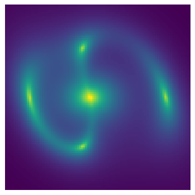
Plot the Results!#
This section is mostly self explanatory. We evaluate the simulator configuration by calling it like a function.
image = sim(x)

plt.imshow(image, origin="lower")
plt.axis("off")
plt.show()
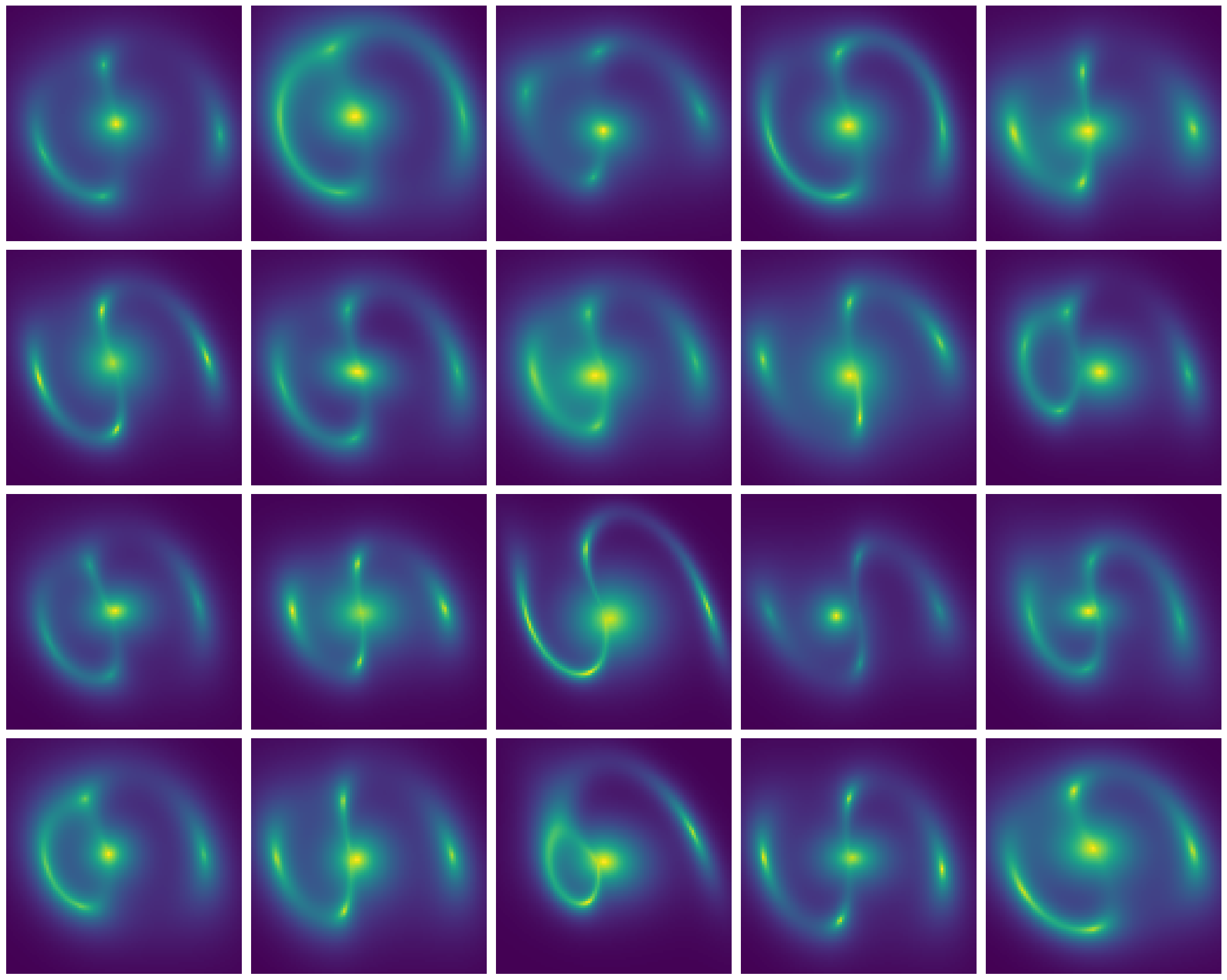
Sampling with a Simulator#
Now let’s see how to use some of the powerful features of the simulator we have created. Note that it behaves essentially like a function, allowing us to take advantage of many JAX features. To start, lets see how we can run batches of lens simulations using vmap.
JAX note Random numbers work differently in JAX than they do for PyTorch or numpy. We have to make a key in order to sample from a random distribution. Most caustics functions are deterministic, for ones that do require randomness, a random key will automatically be generated, but this can be set by the user if needed.
newx = jnp.tile(x, (20, 1))
key = jax.random.PRNGKey(0)
key, subkey = jax.random.split(key)
newx += jax.random.normal(subkey, shape=newx.shape) * 0.1

images = jax.vmap(sim)(newx)

fig, axarr = plt.subplots(4, 5, figsize=(20, 16))
for ax, im in zip(axarr.flatten(), images):
    ax.imshow(im, origin="lower")
    ax.axis("off")
plt.tight_layout()
plt.show()
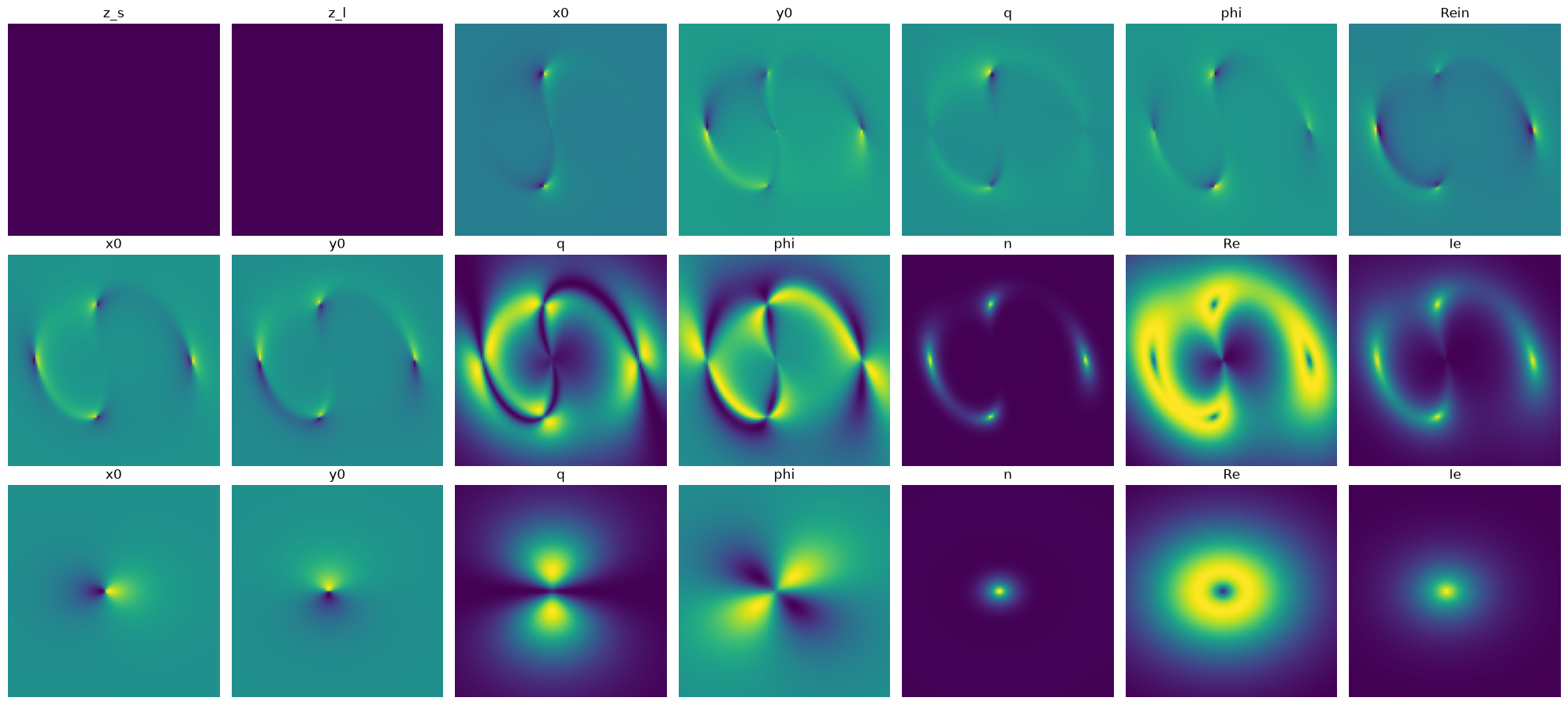
Gradients with autodiff#
Batching is useful for fully parallelizing code and maximally using computational resources, but autodiff gradients allow whole new algorithms and techniques to be used in gravitational lensing! Let’s try computing the Jacobian for the lensing configuration that we have been using so far. The result is a grid of images that show how the lensing simulation image would change if we adjusted each parameter individually. Thanks to autodiff, these derivatives have no finite differences approximation error, they are exact up to the machine precision.
# Now lets compute the jacobian of the simulator wrt each parameter
J = jax.jacfwd(sim)(x)
# The shape of J is (npixels y, npixels x, nparameters)
The Simulator Graph#
Here we take a quick look at the simulator graph for the image we have produced. You will learn much more about what this means in the Simulators tutorial notebook, but let’s cover the basics here. First, note that this is a Directed Acyclic Graph (DAG), this is how all simulator parameters are represented in caustics. At the top of the graph is the LensSource object, you can see in brackets it has a name sim which is used as the identifier for it’s node in the graph. At the next level is the z_s parameter for the redshift of the source. Next are the SIE lens, Sersic source, and Sersic lenslight objects which themselves each hold parameters. You will notice that all the parameters are in white boxes right now, this is because they are dynamic parameters which need values to be passed, grey boxes are used for parameters with fixed values.
# Substitute sim with sim for the yaml method
sim.graphviz()

Model Parameters#
Each of the lens, source, and lenslight models have their own parameters that are needed to sample a given lensing configuration. There are a number of ways to pass these parameters to a caustics simulator, but the most straightforward for most purposes is as a JAX Array.
In order, here is an explanation of the parameters.
z_sis the redshift of the source.z_lis the lens redshift which tells the lens how far away it is from the observer (us).The next two parameters
x0andy0indicate where the lens is relative to the main optical axis, which is the coordinates(0, 0).The
qparameter gives the axis ratio for theSIE, so it knows how elongated it is.phiindicates the position angle (where the ellipse is pointing).Reingives the Einstein radius (in arcsec) of the lens.The next
x0andy0provide the position relative to the main optical axis of the Sersic source, here we offset the source slightly to make for an interesting figure.The
qparameter defines the axis ratio of the Sersic ellipse.phidefines the position angle of the ellipse.nis the Sersic index which determines how concentrated the light is;n=0.5is a Gaussian distribution,n=1is an exponential,n=4is a De Vaucouleurs profile.Reis the radius (in arcsec) within which half the total light of the profile is enclosed.Ieis the brightness atRe.The next set of parameters are also Sersic parameters, but this time they are for the lens light model.