A Menagerie of Lenses#
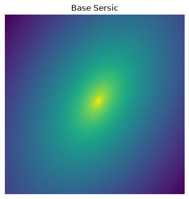
Here we have a quick visual demo of every type of lens in caustics. This is a good way to pick out what you need and quickly copy paste. For all of these lenses we have placed a Sersic source with the same parameters as the background, that way you can visualize the differences between them.
%load_ext autoreload
%autoreload 2

import torch
from torch.nn.functional import avg_pool2d
import matplotlib.pyplot as plt
import numpy as np

import caustics
cosmology = caustics.FlatLambdaCDM()
cosmology.to(dtype=torch.float32)
z_s = torch.tensor(1.0)
z_l = torch.tensor(0.5, dtype=torch.float32)
base_sersic = caustics.Sersic(
    x0=0.1,
    y0=0.1,
    q=0.6,
    phi=np.pi / 3,
    n=2.0,
    Re=1.0,
    Ie=1.0,
)
n_pix = 100
res = 0.05
upsample_factor = 2
fov = res * n_pix
thx, thy = caustics.utils.meshgrid(
    res / upsample_factor,
    upsample_factor * n_pix,
    dtype=torch.float32,
)

plt.imshow(np.log10(base_sersic.brightness(thx, thy).numpy()), origin="lower")
plt.gca().axis("off")
plt.title("Base Sersic")
plt.show()
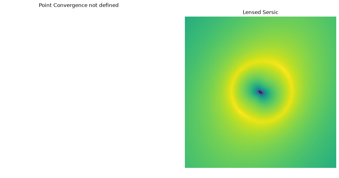
Point (Point)#
The simplest lens, an infinitely small point of mass (did someone say black holes?).
lens = caustics.Point(
    cosmology=cosmology,
    x0=0.0,
    y0=0.0,
    Rein=1.0,
    z_l=z_l,
    z_s=z_s,
)
sim = caustics.LensSource(
    lens=lens,
    source=base_sersic,
    pixelscale=res,
    pixels_x=n_pix,
    upsample_factor=2,
)
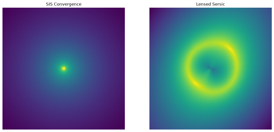
Singular Isothermal Sphere (SIS)#
An SIS is a mass distribution represented by a constant temperature velocity dispersion of masses. Alternatively, a constant temperature gas in a spherical gravitational potential.
lens = caustics.SIS(
    cosmology=cosmology,
    x0=0.0,
    y0=0.0,
    Rein=1.0,
    z_l=z_l,
    z_s=z_s,
)
sim = caustics.LensSource(
    lens=lens,
    source=base_sersic,
    pixelscale=res,
    pixels_x=n_pix,
    upsample_factor=2,
)
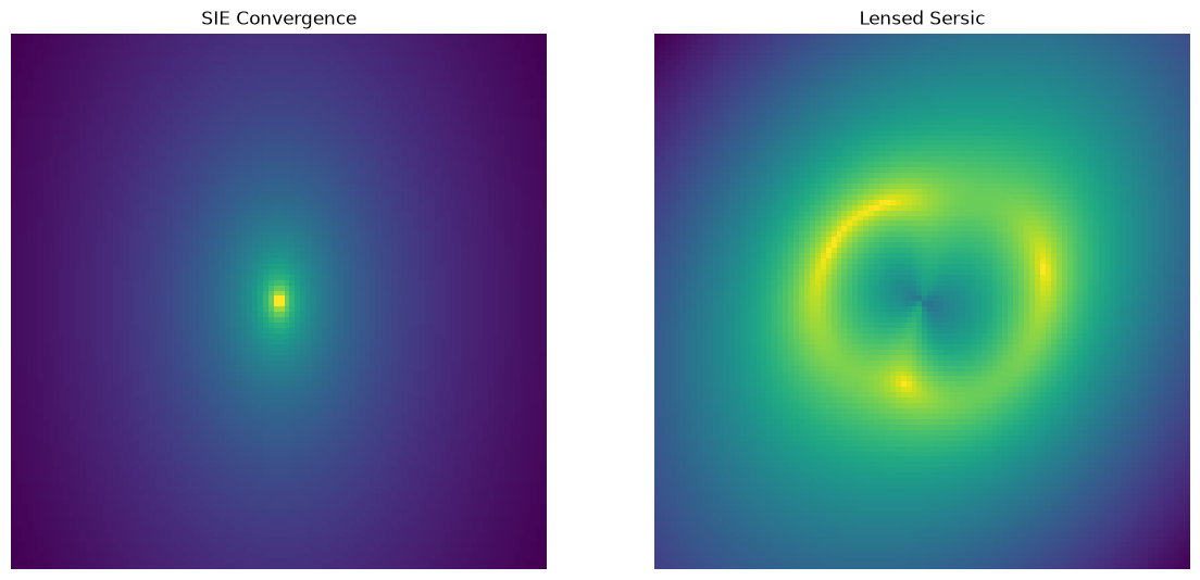
Singular Isothermal Ellipsoid (SIE)#
The SIE is just like the SIS except it has been compressed along one axis.
lens = caustics.SIE(
    cosmology=cosmology,
    x0=0.0,
    y0=0.0,
    q=0.6,
    phi=np.pi / 2,
    Rein=1.0,
    z_l=z_l,
    z_s=z_s,
)
sim = caustics.LensSource(
    lens=lens,
    source=base_sersic,
    pixelscale=res,
    pixels_x=n_pix,
    upsample_factor=2,
)
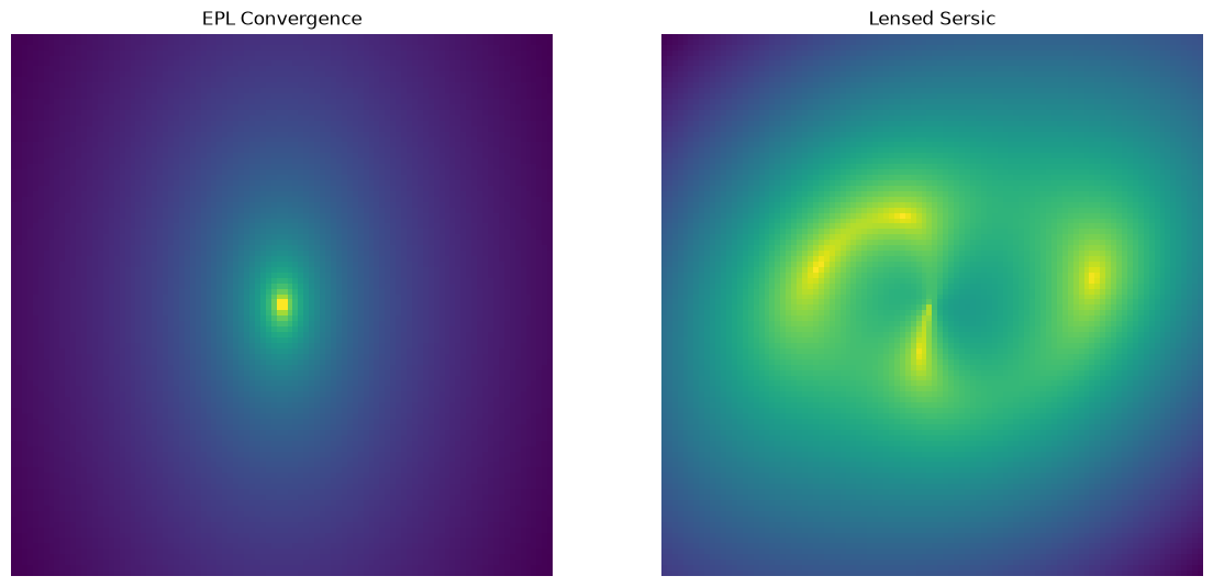
Elliptical Power Law (EPL)#
This is a power law mass distribution with an elliptical isodensity contour.
lens = caustics.EPL(
    cosmology=cosmology,
    x0=0.0,
    y0=0.0,
    q=0.6,
    phi=np.pi / 2,
    Rein=1.0,
    t=0.5,
    z_l=z_l,
    z_s=z_s,
)
sim = caustics.LensSource(
    lens=lens,
    source=base_sersic,
    pixelscale=res,
    pixels_x=n_pix,
    upsample_factor=2,
)
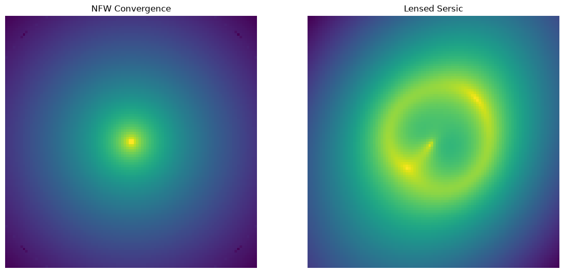
Navarro Frenk White profile (NFW)#
The NFW profile is a classic mass profile that approximates the mass distribution of halos in large dark matter simulations.
lens = caustics.NFW(
    cosmology=cosmology,
    x0=0.0,
    y0=0.0,
    mass=1e13,
    c=20.0,
    z_l=z_l,
    z_s=z_s,
)
sim = caustics.LensSource(
    lens=lens,
    source=base_sersic,
    pixelscale=res,
    pixels_x=n_pix,
    upsample_factor=2,
)
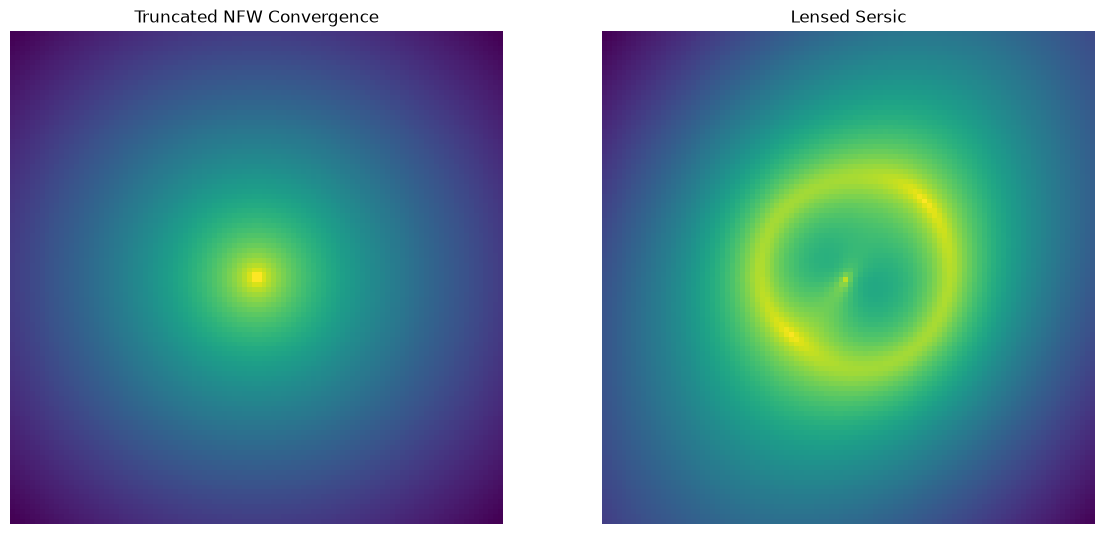
Truncated NFW profile (TNFW)#
The TNFW profile is a slight modification to the classic NFW mass profile that approximates the mass distribution of halos in large dark matter simulations. The new density profile is defined as:
where \(\tau = \frac{r_t}{r_s}\) is the ratio of the truncation radius to the scale radius. Note that the truncation happens smoothly so there are no sharp boundaries. In the TNFW profile, the mass quantity now actually corresponds the to the total mass since it is no longer divergent. This often means the mass values are larger.
lens = caustics.TNFW(
    cosmology=cosmology,
    x0=0.0,
    y0=0.0,
    mass=1e12,
    Rs=1.0,
    tau=3.0,
    z_l=z_l,
    z_s=z_s,
)
sim = caustics.LensSource(
    lens=lens,
    source=base_sersic,
    pixelscale=res,
    pixels_x=n_pix,
    upsample_factor=2,
)
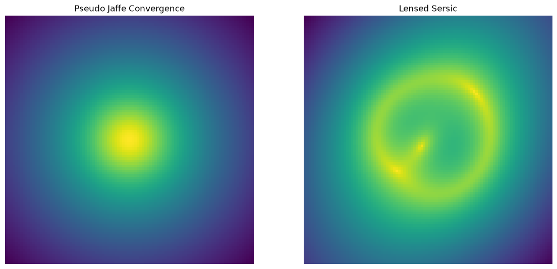
Pseudo Jaffe (PseudoJaffe)#
The Pseudo Jaffe closely approximates an isothermal mass distribution except that it is easier to compute and has finite mass.
where \(\rho_0\) is the central density limit, \(r_c\) is the core radius, \(r_s\) is the scale radius.
lens = caustics.PseudoJaffe(
    cosmology=cosmology,
    x0=0.0,
    y0=0.0,
    mass=1e13,
    Rc=5e-1,
    Rs=15.0,
    z_l=z_l,
    z_s=z_s,
)
sim = caustics.LensSource(
    lens=lens,
    source=base_sersic,
    pixelscale=res,
    pixels_x=n_pix,
    upsample_factor=2,
)
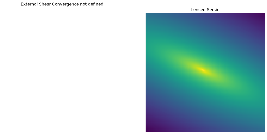
External Shear (ExternalShear)#
It is often necessary to embed a lens in an external shear field to account for the fact that the lensing mass is not the only mass in the universe.
lens = caustics.ExternalShear(
    cosmology=cosmology,
    x0=0.0,
    y0=0.0,
    gamma_1=1.0,
    gamma_2=-1.0,
    z_l=z_l,
    z_s=z_s,
)
sim = caustics.LensSource(
    lens=lens,
    source=base_sersic,
    pixelscale=res,
    pixels_x=n_pix,
    upsample_factor=2,
)
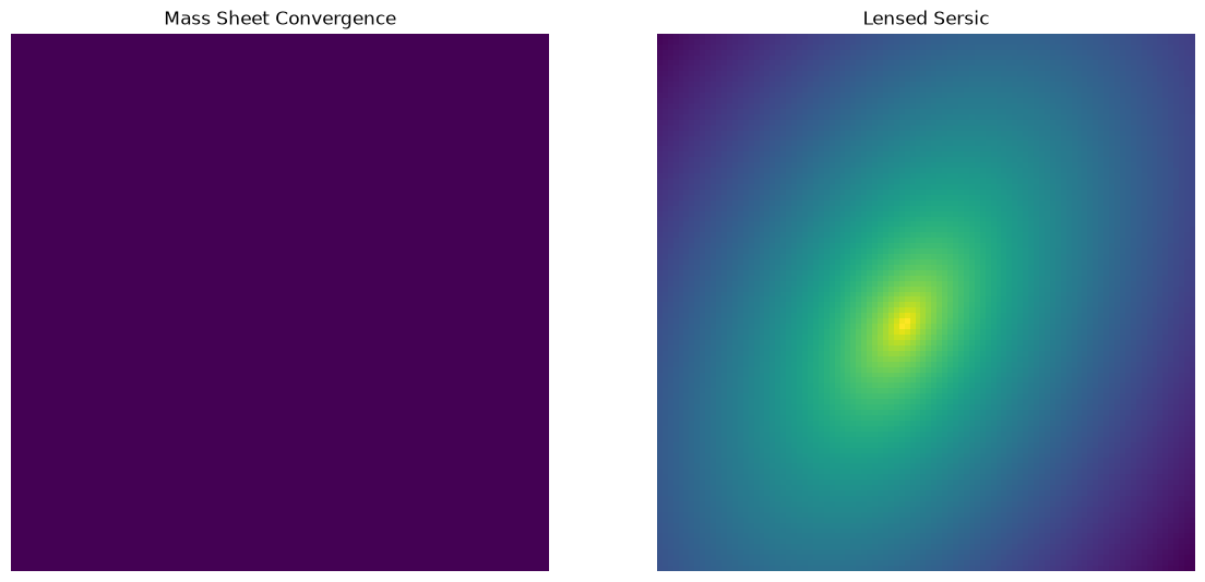
Mass Sheet (MassSheet)#
This is a simple case of an external shear field which represents an infinite constant surface density sheet.
lens = caustics.MassSheet(
    cosmology=cosmology,
    x0=0.0,
    y0=0.0,
    kappa=1.5,
    z_l=z_l,
    z_s=z_s,
)
sim = caustics.LensSource(
    lens=lens,
    source=base_sersic,
    pixelscale=res,
    pixels_x=n_pix,
    upsample_factor=2,
)
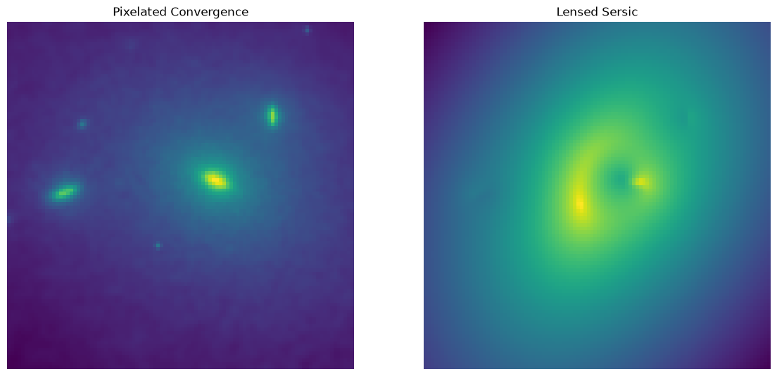
Pixelated Convergence (PixelatedConvergence)#
This is an image which can be used to represent the convergence field of a mass distribution. Typically this is useful for taking n-body simulations and using them for lensing, or when using machine learning.
kappa_map = np.load("assets/kappa_maps.npz", allow_pickle=True)["kappa_maps"][1]

lens = caustics.PixelatedConvergence(
    cosmology=cosmology,
    x0=0.0,
    y0=0.0,
    convergence_map=kappa_map,
    pixelscale=res,
    z_l=z_l,
    z_s=z_s,
)
sim = caustics.LensSource(
    lens=lens,
    source=base_sersic,
    pixelscale=res,
    pixels_x=n_pix,
    upsample_factor=2,
)
fig, axarr = plt.subplots(1, 2, figsize=(14, 7))
convergence = avg_pool2d(
    lens.convergence(thx, thy).squeeze()[None, None], upsample_factor
).squeeze()
axarr[0].imshow(np.log10(convergence.numpy()), origin="lower")
axarr[0].axis("off")
axarr[0].set_title("Pixelated Convergence")
axarr[1].imshow(np.log10(sim().numpy()), origin="lower")
axarr[1].axis("off")
axarr[1].set_title("Lensed Sersic")
plt.show()
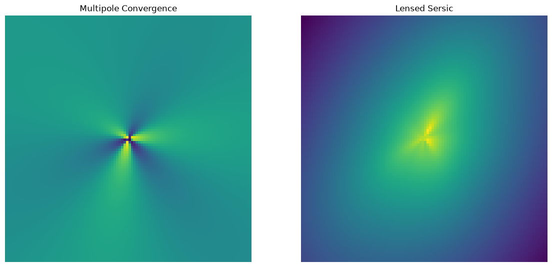
Multipole (Multipole)#
This is a lens type typically used to add a perturbation to another lens. Higher order multipoles allow for more complex perturbations.
lens = caustics.Multipole(
    cosmology=cosmology,
    x0=0.0,
    y0=0.0,
    m=(3, 4),
    a_m=(0.5, 0.25),
    phi_m=(0.25, -0.125),
    z_l=z_l,
    z_s=z_s,
)
sim = caustics.LensSource(
    lens=lens,
    source=base_sersic,
    pixelscale=res,
    pixels_x=n_pix,
    upsample_factor=2,
)
fig, axarr = plt.subplots(1, 2, figsize=(14, 7))
convergence = avg_pool2d(
    lens.convergence(thx, thy).squeeze()[None, None], upsample_factor
).squeeze()
axarr[0].imshow(np.arctan(convergence.numpy()), origin="lower")
axarr[0].axis("off")
axarr[0].set_title("Multipole Convergence")
axarr[1].imshow(np.log10(sim().numpy()), origin="lower")
axarr[1].axis("off")
axarr[1].set_title("Lensed Sersic")
plt.show()