import caustics
from caustics import Module, forward, Param
from torch.nn.functional import conv2d, avg_pool2d
import numpy as np
import torch
from torch import pi
import matplotlib.pyplot as plt
Building your own simulator from scratch: a tutorial#
In this tutorial, we will build a fully-functional gravitational lensing simulator based on LensSource, the prebuilt simulator which comes with caustics. We will then demonstrate how you can modify a custom simulator to extend its capabilities.
Part 1: The __init__ function#
First, we begin by creating a new class for our simulator.
For those new to object-oriented programming: a class is like a dictionary, you can store anything in it and retrieve it by name. The syntax is a bit different, instead of doing dictionary["key"] to get something from it, you would do instance.attribute to access that value, function, or even another class instance. When you write a class it is like a template, you need to instantiate the template (something like myinstance = myclass(initial, parameters)) to get an object that you can use.
We want our simulator to inherit from the Module class in caustics, which is a basic framework for constructing simulator objects. To create inheritance, we put the parent class as an argument (in parentheses) to the child class. Then, in the __init__ function, we need a few basic ingredients to create the simulator:
A lens mass distribution
A model for the lens light
A model for the source light
A model for the telescope PSF
A value for the pixel scale of the CCD
The number of pixels in the CCD
The upsample factor (increases the resolution of the simulator internally to improve accuracy)
We can also provide a name for the simulator.
Within our __init__ function, we need to provide instructions to construct the basic structure of the simulator object, which is done by calling the __init__ function of the super class, which in this case is Module from caustics.
Within __init__ we also need to construct the components of our simulator. For components which are constructed once (lens mass model, lens light model, and source light model), we simply need to make them attributes of the current object being constructed (self). We do the same for parameters whose value we wish to only set once, such as the coordinate grid, which we generate with the meshgrid function of caustics. For parameters which we wish to sample with our MCMC (which are not already parameters of any of the existing components), we need to register them as a Param object, which will allow our simulator to find them in the flattened vector of parameters which we will pass to the simulator. In this example, we register the PSF as a Param and name it "PSF". We also have to tell Param what shape the PSF array will take so that the PSF can be extracted from the flattened tensor (in this example, we allow a variable-sized PSF). For more information on the underlying functionality of Module, Param, and related parameter handling capabilities in caustics, see the underlying caskade package and associated documentation: https://caskade.readthedocs.io/en/latest/notebooks/BeginnersGuide.html
class Singlelens(Module):
    def __init__(
        self,
        lens,
        lens_light,
        source,
        pixelscale,
        pixels_x,
        upsample_factor,
        psf=None,
        name: str = "sim",
    ):
        super().__init__(name)

        self.lens = lens
        self.src = source
        self.lens_light = lens_light
        self.psf = Param("PSF", psf)
        self.upsample_factor = upsample_factor

        # Create the high-resolution grid
        thx, thy = caustics.utils.meshgrid(
            pixelscale / upsample_factor,
            upsample_factor * pixels_x,
            dtype=torch.float32,
        )

        self.thx = thx
        self.thy = thy

    @forward
    def run_simulator(self, psf):
        # Ray-trace to get the lensed positions
        bx, by = self.lens.raytrace(self.thx, self.thy)

        # Evaluate the lensed source brightness at high resolution
        image = self.src.brightness(bx, by)

        # Add the lens light
        image += self.lens_light.brightness(self.thx, self.thy)

        # Downsample to the desired resolution
        image_ds = avg_pool2d(image[None, None], self.upsample_factor)[0, 0]

        # Convolve with the PSF using conv2d
        psf_normalized = (psf.T / psf.sum())[None, None]
        image_ds = (
            conv2d(image_ds[None, None], psf_normalized, padding="same")
            .squeeze(0)
            .squeeze(0)
        )

        return image_ds
Part 2: the @forward-decorated function#
In the code above, in addition to the __init__ function, you can see that we have added another function called run_simulator. This is the part of our simulator object which will actually perform the simulation (when called). Our simulation has a few basic steps:
Raytrace the coordinate grid backwards from the lens plane (
thx,thy) to the source plane (bx,by) using the lens mass distribution. This produces the source plane coordinates at the corresponding locations in the lens plane.Evaluate the brightness of the source light model at the raytraced coordinates (which creates the gravitationally lensed image)
Add lens light to the image, sampled directly at
thx,thyDownsample the image to the correct pixel scale
Convolve with the PSF of the telescope
To ensure that all the Param parameters in the simulator are handled correctly, we need to add the @forward decorator from caustics (which is just the @forward decorator from caskade) to our run_simulator function. Note that since psf is a Param of our simulator, we won’t need to pass it directly when calling run_simulator, instead it will be extracted from the params tensor (see part 4).
Part 3: Instantiating our simulator#
Now that we have completed our custom simulator, we need to instantiate the components of the simulator and the simulator itself. The instantiation process creates an object in memory from a class.
# Cosmology model
cosmology = caustics.FlatLambdaCDM(name="cosmo")
# Source light model
source_light = caustics.Sersic(
    name="sourcelight",
    x0=0.25,
    y0=0.3,
    q=1 - 0.29,
    phi=-30 * pi / 180,
    n=4,
    Re=0.1,
    Ie=36,
)
# Lens mass model
epl = caustics.EPL(
    name="epl",
    cosmology=cosmology,
    z_s=3.5,
    z_l=1.5,
    x0=0.25,
    y0=0.3,
    q=1 / 1.14,
    phi=pi / 2 + 1.6755160819145565,
    Rein=1.036,
    t=1.04,
)
# Lens Light model
lens_light = caustics.Sersic(
    name="lenslight1",
    x0=0.25,
    y0=0.3,
    q=1 - 0.29,
    phi=-30 * pi / 180,
    n=4,
    Re=0.1,
    Ie=100,
)
# PSF and image resolution
pixscale = 0.11 / 2
fwhm = 0.269  # full width at half maximum of PSF
psf_sigma = fwhm / (2 * np.sqrt(2 * np.log(2)))
n_psf = 11
psf_image = caustics.utils.gaussian(
    nx=n_psf,
    ny=n_psf,
    pixelscale=pixscale,
    sigma=psf_sigma,
    upsample=1,
)
# Instantiate simulator
simulator = Singlelens(
    lens=epl,
    lens_light=lens_light,
    source=source_light,
    pixels_x=60 * 2,
    pixelscale=pixscale,
    upsample_factor=5,
    psf=psf_image,
)
# Set all parameters to be dynamic
simulator.to_dynamic(children_only=False)
cosmology.to_static()  # except cosmology parameters
Now that we have instantiated our simulator, we can visualize its structure using graphviz. The grayed out squares are parameters which are fixed (known as static parameters in caustics), while the white squares are parameters whose value will be set once the forward function is run (these are known as dynamic parameters in caustics). The arrows indicate which object contains which component.
simulator.graphviz()

Part 4: Passing parameters to our simulator#
Now that we have designed our simulator class and instantiated our simulator object, we can use the forward method to run the simulator. Thanks to caskade, we can pass all of the dynamic parameters at once as a flattened Pytorch tensor. However, we need to know what order to put our parameters in the tensor. We can find the order by literally printing our simulator:
print(simulator)
sim|Singlelens
    epl|EPL
        cosmo|FlatLambdaCDM
            h0|static: 0.677
            critical_density_0|static: 1.27e+11
            Om0|static: 0.31
        z_s|dynamic: 3.5
        z_l|dynamic: 1.5
        x0|dynamic: 0.25
        y0|dynamic: 0.3
        q|dynamic: 0.877
        phi|dynamic: 3.25
        Rein|dynamic: 1.04
        t|dynamic: 1.04
    sourcelight|Sersic
        x0|dynamic: 0.25
        y0|dynamic: 0.3
        q|dynamic: 0.71
        phi|dynamic: -0.524
        n|dynamic: 4
        Re|dynamic: 0.1
        Ie|dynamic: 36
    lenslight1|Sersic
        x0|dynamic: 0.25
        y0|dynamic: 0.3
        q|dynamic: 0.71
        phi|dynamic: -0.524
        n|dynamic: 4
        Re|dynamic: 0.1
        Ie|dynamic: 100
    PSF|dynamic: (11, 11)
In truth, we don’t need to make the tensor ourselves. In part 3 we assigned a value to all of the parameters before using to_dynamic to set which parameters would be free to vary, these values are remembered by the Param objects. Since every parameter remembers its starting value, it can build the tensor on its own (very helpful as simulators get complicated!).
# Now create a flattened tensor
params_for_simulator = simulator.get_values()
print("Params tensor shape: ", params_for_simulator.shape)
Params tensor shape: torch.Size([143])
Each of the pixel values in the PSF is now an independent parameter which can be jointly sampled alongside the other parameters! The PSF, just like all the other dynamic parameters, will be pulled out of this big flattened tensor and reshaped to what it should be (a square 2D tensor for PSF) before going into the simulation.
Now we can run our simulator by passing the flat parameter tensor to the forward function:
lensed_image = simulator.run_simulator(params_for_simulator)
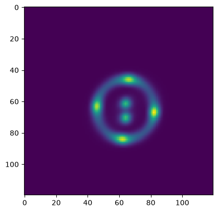
We can then view the lensed image output by our simulator (here we have created an “Einstein cross”):
plt.imshow(lensed_image)
plt.show()
A final word on why we would want to do this, it seems like a lot of work to flatten and combine all the parameters into a single large tensor, just to break it up and reshape everything back to its original state. The reason is that a lot of other codes (think MCMC samplers and optimizers) really prefer to work with a simple 1D vector when performing their tasks. You can now automatically interface with essentially any 3rd party code no matter how complex your simulator becomes. This turns out to be really powerful!
Part 5: Customizing your simulator#
So far, we have focused on re-creating the LensSource simulator provided by default in caustics, but the real power of the caustics package is reflected by its extensibility.
Suppose we want to have a single background light source and a single lens mass distribution, but instead of a single lens light source, we want two lens light sources (this could be a modeling choice for merging lensed galaxies).
We can implement this by creating a new simulator class, which we will call Doublelenslight. This class is identical to Singlelens, except for two things: we add an extra lens_light to our __init__, and in the forward we add the second lens_light to the image.
class Doublelenslight(Module):
    def __init__(
        self,
        lens,
        lens_light1,
        lens_light2,  # NEW!
        source,
        pixelscale,
        pixels_x,
        upsample_factor,
        psf=None,
        name: str = "sim",
    ):
        super().__init__(name)

        self.lens = lens
        self.src = source
        self.lens_light1 = lens_light1
        self.lens_light2 = lens_light2  # NEW!
        self.psf = Param("psf", psf)
        self.upsample_factor = upsample_factor

        # Create the high-resolution grid
        thx, thy = caustics.utils.meshgrid(
            pixelscale / upsample_factor,
            upsample_factor * pixels_x,
            dtype=torch.float32,
        )

        self.thx = thx
        self.thy = thy

    @forward
    def run_simulator(self, psf):
        # Ray-trace to get the lensed positions
        bx, by = self.lens.raytrace(self.thx, self.thy)

        # Evaluate the lensed source brightness at high resolution
        image = self.src.brightness(bx, by)

        # Add the lens light
        image += self.lens_light1.brightness(self.thx, self.thy)
        image += self.lens_light2.brightness(self.thx, self.thy)  # NEW!

        # Downsample to the desired resolution
        image_ds = avg_pool2d(image[None, None], self.upsample_factor)[0, 0]

        # Convolve with the PSF using conv2d
        psf_normalized = (psf.T / psf.sum())[None, None]
        image_ds = (
            conv2d(image_ds[None, None], psf_normalized, padding="same")
            .squeeze(0)
            .squeeze(0)
        )

        return image_ds
# Cosmology model
cosmology = caustics.FlatLambdaCDM(name="cosmo")
# Source light model
source_light = caustics.Sersic(
    name="sourcelight",
    x0=0.25,
    y0=0.3,
    q=1 - 0.29,
    phi=-30 * pi / 180,
    n=4,
    Re=0.1,
    Ie=36,
)
# Lens mass model
epl = caustics.EPL(
    name="epl",
    cosmology=cosmology,
    z_s=3.5,
    z_l=1.5,
    x0=0.25,
    y0=0.3,
    q=1 / 1.14,
    phi=pi / 2 + 1.6755160819145565,
    Rein=1.036,
    t=1.04,
)
# Lens Light models
lens_light1 = caustics.Sersic(
    name="lenslight1",
    x0=0.25,
    y0=0.1,
    q=1 - 0.29,
    phi=-30 * pi / 180,
    n=4,
    Re=0.1,
    Ie=100,
)
lens_light2 = caustics.Sersic(
    name="lenslight2",
    x0=0.25,
    y0=0.6,
    q=1 - 0.29,
    phi=-30 * pi / 180,
    n=4,
    Re=0.1,
    Ie=100,
)
# PSF and image resolution
pixscale = 0.11 / 2
fwhm = 0.269  # full width at half maximum of PSF
psf_sigma = fwhm / (2 * np.sqrt(2 * np.log(2)))
n_psf = 11
psf_image = caustics.utils.gaussian(
    nx=n_psf,
    ny=n_psf,
    pixelscale=pixscale,
    sigma=psf_sigma,
    upsample=1,
)
# Instantiate simulator
simulator = Doublelenslight(
    lens=epl,
    lens_light1=lens_light1,
    lens_light2=lens_light2,
    source=source_light,
    pixels_x=60 * 2,
    pixelscale=pixscale,
    upsample_factor=5,
    psf=psf_image,
)
simulator.to_dynamic(children_only=False)
cosmology.to_static()
# Note we can also flip individual parameters between dynamic and static
epl.z_s.to_static()
epl.z_l.to_static()
simulator.graphviz()

When passing parameters to the forward, we need to use
print(simulator)
sim|Doublelenslight
    epl|EPL
        cosmo|FlatLambdaCDM
            h0|static: 0.677
            critical_density_0|static: 1.27e+11
            Om0|static: 0.31
        z_s|static: 3.5
        z_l|static: 1.5
        x0|dynamic: 0.25
        y0|dynamic: 0.3
        q|dynamic: 0.877
        phi|dynamic: 3.25
        Rein|dynamic: 1.04
        t|dynamic: 1.04
    sourcelight|Sersic
        x0|dynamic: 0.25
        y0|dynamic: 0.3
        q|dynamic: 0.71
        phi|dynamic: -0.524
        n|dynamic: 4
        Re|dynamic: 0.1
        Ie|dynamic: 36
    lenslight1|Sersic
        x0|dynamic: 0.25
        y0|dynamic: 0.1
        q|dynamic: 0.71
        phi|dynamic: -0.524
        n|dynamic: 4
        Re|dynamic: 0.1
        Ie|dynamic: 100
    lenslight2|Sersic
        x0|dynamic: 0.25
        y0|dynamic: 0.6
        q|dynamic: 0.71
        phi|dynamic: -0.524
        n|dynamic: 4
        Re|dynamic: 0.1
        Ie|dynamic: 100
    psf|dynamic: (11, 11)
params_for_simulator = simulator.get_values()
lensed_image = simulator.run_simulator(params_for_simulator)
# Note the params object can be a tensor, list, or dictionary
# The dictionary option is the most human readable
params_dict = simulator.get_values("dict")
params_dict.pop("psf")  # this one is big because of the PSF
print(params_dict)
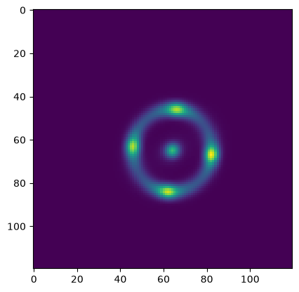
{'lens': {'x0': tensor(0.2500), 'y0': tensor(0.3000), 'q': tensor(0.8772), 'phi': tensor(3.2463), 'Rein': tensor(1.0360), 't': tensor(1.0400)}, 'src': {'x0': tensor(0.2500), 'y0': tensor(0.3000), 'q': tensor(0.7100), 'phi': tensor(-0.5236), 'n': tensor(4), 'Re': tensor(0.1000), 'Ie': tensor(36)}, 'lens_light1': {'x0': tensor(0.2500), 'y0': tensor(0.1000), 'q': tensor(0.7100), 'phi': tensor(-0.5236), 'n': tensor(4), 'Re': tensor(0.1000), 'Ie': tensor(100)}, 'lens_light2': {'x0': tensor(0.2500), 'y0': tensor(0.6000), 'q': tensor(0.7100), 'phi': tensor(-0.5236), 'n': tensor(4), 'Re': tensor(0.1000), 'Ie': tensor(100)}}
plt.imshow(lensed_image)
plt.show()