Fit Lens to QSO positions

In this hypothetical scenario we are observing a quadrouply lensed Quasar and we would like to learn something about the Lens mass distribution causing the strong gravitational lensing. Since each QSO image is a point source, we can determine its position with high precision (sub pixel level accuracy), so we would like to use the four positions to recover the parameters of an SIE mass profile.

%load_ext autoreload
%autoreload 2


import torch
import matplotlib.pyplot as plt
import numpy as np

import caustics

First lets create the lens we intend to fit. In this case it is an SIE model. The SIE parameters are unknown at this point so this is just a generic SIE model.

cosmology = caustics.FlatLambdaCDM(name="cosmo")
cosmology.to(dtype=torch.float32)

z_l = torch.tensor(0.5, dtype=torch.float32)
z_s = torch.tensor(1.5, dtype=torch.float32)
lens = caustics.SIE(
    cosmology=cosmology,
    name="sie",
    z_l=z_l,
    z_s=z_s,
    x0=0.0,
    y0=0.0,
    q=0.4,
    phi=np.pi / 5,
    Rein=1.0,
    s=1e-3,
)
for p in ["x0", "y0", "q", "phi", "Rein"]:
    lens[p].to_dynamic()

To create a mock dataset to try and fit, we choose a source position and lens parameters then forward raytrace to find the image plane positions.

# Point in the source plane
sp_x = torch.tensor(0.2)
sp_y = torch.tensor(0.2)

#  true parameters
params = lens.get_values()
# Points in image plane
x, y = lens.forward_raytrace(sp_x, sp_y, params)
# get magnifications
mu = lens.magnification(x, y, params)
# remove heavily demagnified points
x = x[mu > 1e-2]
y = y[mu > 1e-2]

Just to see what’s going on, we plot the caustics and image/source plane positions.

n_pix = 100
res = 0.05
upsample_factor = 1
fov = res * n_pix
thx, thy = caustics.utils.meshgrid(
    res / upsample_factor,
    upsample_factor * n_pix,
    dtype=torch.float32,
)

A = lens.jacobian_lens_equation(thx, thy, params)
detA = torch.linalg.det(A)

Show code cell source

Hide code cell source

fig, ax = plt.subplots()
CS = ax.contour(thx, thy, detA, levels=[0.0], colors="b", zorder=1)
# Get the path from the matplotlib contour plot of the critical line
paths = CS.allsegs[0]
caustic_paths = []
for path in paths:
    # Collect the path into a discrete set of points
    x1 = torch.tensor(list(float(vs[0]) for vs in path))
    x2 = torch.tensor(list(float(vs[1]) for vs in path))
    # raytrace the points to the source plane
    y1, y2 = lens.raytrace(x1, x2, params)

    # Plot the caustic
    ax.plot(y1, y2, color="r", zorder=1)
ax.scatter(x, y, color="b", label="forward raytrace", zorder=10)
ax.scatter(sp_x, sp_y, color="r", marker="x", label="source plane", zorder=9)
plt.legend()
plt.show()

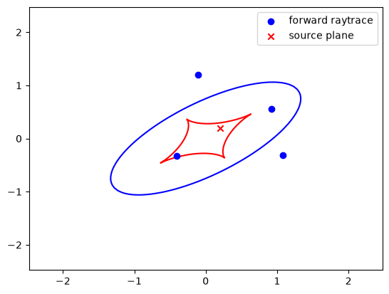
In this experiment we have access to the image plane positions x and y (the blue dots) but we will assume we don’t know the source plane position (red x) or the lens model parameters (x0, y0, q, phi, b). Let’s start from some slightly incorrect parameters and try to recover the true parameters.

The function we will try to optimize is determined by raytracing the four points back to the source plane. We assume that the four QSO images all came from the same place, so when we find SIE parameters which map the four images back to the same spot then we have found some valid SIE parameters!

In this example we run from 50 random starting points and let the Levenberg Marquardt try to find lensing parameters which map the image positions to a single source position. After the optimization finishes, we select which run actually ended up finding parameters that converge the source positions. The resulting parameters are incredibly close to the true values!

init_params = params.repeat(50, 1)
init_params += torch.normal(mean=0.0, std=0.1 * torch.ones_like(init_params))


# Compute Chi^2 which is just the distance between the four images raytraced back to the source plane.
# This returns zero when all QSO images land in the same spot.
def loss(P):
    bx, by = lens.raytrace(x, y, P)
    return torch.cat(
        (
            torch.sum((bx[0] - bx[1:]) ** 2).unsqueeze(-1),
            torch.sum((by[0] - by[1:]) ** 2).unsqueeze(-1),
        )
    )


fit_params = caustics.utils.batch_lm(
    init_params, torch.zeros(init_params.shape[0], 2), loss, stopping=1e-8
)
# Fit params includes:
# The fitted parameter values, A levenberg-marquardt damping parameter, the chi^2 values

# Here we print the parameter values that have a good chi^2
# If you decrease the threshold from 1e-8 to 1e-10 you will get better fits, but fewer of them
avg_fit = torch.mean(fit_params[0][fit_params[2] < 1e-8], dim=0)
print(avg_fit.numpy())
# Note that the order is: x0, y0, q, phi, Rein

[0.00335226 0.00295409 0.40309146 0.6283246  0.9987042 ]

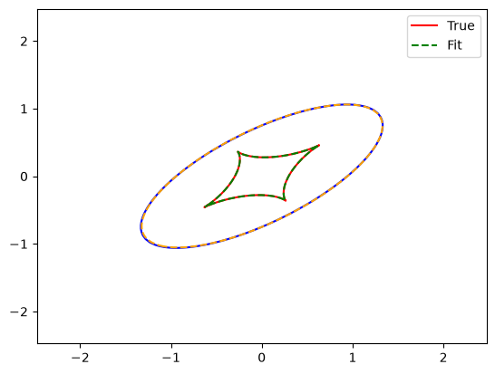
Next we plot a comparison of the true lensing parameters and the fitted parameters. The fit is so good we used dashed lines so you can see the ground truth underneath!

Show code cell source

Hide code cell source

fig, ax = plt.subplots()

# Plot True caustics
###############
CS = ax.contour(thx, thy, detA, levels=[0.0], colors="b", zorder=1)
# Get the path from the matplotlib contour plot of the critical line
paths = CS.allsegs[0]
caustic_paths = []
for path in paths:
    # Collect the path into a discrete set of points
    x1 = torch.tensor(list(float(vs[0]) for vs in path))
    x2 = torch.tensor(list(float(vs[1]) for vs in path))
    # raytrace the points to the source plane
    y1, y2 = lens.raytrace(x1, x2, params)

    # Plot the caustic
    ax.plot(y1, y2, color="r", label="True", zorder=1)

# Plot fitted caustics
#################

A = lens.jacobian_lens_equation(thx, thy, avg_fit)
detA = torch.linalg.det(A)

CS = ax.contour(
    thx, thy, detA, levels=[0.0], colors="orange", linestyles="dashed", zorder=1
)
# Get the path from the matplotlib contour plot of the critical line
paths = CS.allsegs[0]
caustic_paths = []
for path in paths:
    # Collect the path into a discrete set of points
    x1 = torch.tensor(list(float(vs[0]) for vs in path))
    x2 = torch.tensor(list(float(vs[1]) for vs in path))
    # raytrace the points to the source plane
    y1, y2 = lens.raytrace(x1, x2, params)

    # Plot the caustic
    ax.plot(y1, y2, color="green", linestyle="--", label="Fit", zorder=1)
plt.legend()
plt.show()