Modelling a Lens image using MCMC#
In this hypothetical scenario we have an image of galaxy galaxy strong lensing and we would like to recover a model of this scene. Thus we will need to determine parameters for the background source light, the lensing galaxy light, and the lensing galaxy mass distribution. A common technique for analyzing strong lensing systems is a Markov Chain Monte-Carlo which can explore the parameter space and provide us with important metrics about the model and uncertainty on all parameters. Since caustics is differentiable we have access to especially efficient gradient based MCMC algorithms. First, we will demo a classical MCMC algorithm (using emcee) on the problem and show how for this high dimensional problem the autocorrelation length is high. Next we will show how just adding a bit of gradient information (via MALA) will significantly improve results by reducing autocorrelation length. Finally, we will demo NUTS on the problem, which is highly gradient based and is convenient in that it can be run with no tunable parameters, it’s autocorrelation length is generally approximately 1. However, to achieve this, NUTS needs to run many steps internally, which ultimately means that even though it requires more tweaking to set up, MALA, is often more efficient. The best algorithm for your use case will depend on a number of factors, here you will see how caustics can play well with any sampling algorithm available, giving you lots of flexibility!
import caustics
import numpy as np
import torch
import matplotlib.pyplot as plt
from matplotlib import colormaps
from matplotlib.patches import Ellipse
from scipy.stats import norm
from tqdm.notebook import tqdm

import pyro
import pyro.distributions as dist
from pyro.infer import MCMC as pyro_MCMC
from pyro.infer import NUTS as pyro_NUTS
import emcee
Specs for the data#
These are some properties of the data that aren’t very interesting for the demo, it includes the size of the image, pixelscale, noise level, etc.
Build simulator forward model#
Here we build the caustics simulator which will handle the lensing and generating our images for the sake of fitting. It includes a model for the lens mass distribution, lens light, and source light. We also include a simple gaussian PSF for extra realism, though for simplicity we will use the same PSF model for simulating the mock data and fitting.
# Lens mass model (SIE + shear)
lens_sie = caustics.SIE(
    name="galaxylens",
    cosmology=cosmology,
    x0=0.05,
    y0=0.0,
    q=0.86,
    phi=-0.20,
    Rein=0.66,
)
lens_sie.to_dynamic()

lens_shear = caustics.ExternalShear(
    name="externalshear",
    cosmology=cosmology,
    x0=0.0,
    y0=0.0,
    gamma_1=0.0,
    gamma_2=-0.05,
)
lens_shear.gamma_1.to_dynamic()
lens_shear.gamma_2.to_dynamic()

lens_mass_model = caustics.SinglePlane(
    name="lensmass",
    cosmology=cosmology,
    lenses=[lens_sie, lens_shear],
    z_l=z_l,
    z_s=z_s,
)

# Lens light model (sersic)
lens_light_model = caustics.Sersic(
    name="lenslight",
    x0=0.05,
    y0=0.0,
    q=0.75,
    phi=1.18,
    n=2.0,
    Re=0.6 / np.sqrt(0.75),
    Ie=16 * pixelscale**2,
)
lens_light_model.to_dynamic()

# Source light model (sersic)
source_light_model = caustics.Sersic(
    name="sourcelight",
    x0=0.1,
    y0=0.0,
    q=0.75,
    phi=1.18,
    n=1.0,
    Re=0.1 / np.sqrt(0.75),
    Ie=16 * pixelscale**2,
)
source_light_model.to_dynamic()

# Gaussian PSF Model
psf_image = caustics.utils.gaussian(
    nx=upsample_factor * 6 + 1,
    ny=upsample_factor * 6 + 1,
    pixelscale=pixelscale / upsample_factor,
    sigma=psf_sigma,
    upsample=2,
)

# Image plane simulator
sim = caustics.LensSource(
    lens=lens_mass_model,
    lens_light=lens_light_model,
    source=source_light_model,
    psf=psf_image,
    pixels_x=numPix,
    pixelscale=pixelscale,
    upsample_factor=upsample_factor,
    quad_level=quad_level,
)
sim.to(dtype=torch.float32)
sim.graphviz()

Sample some mock data#
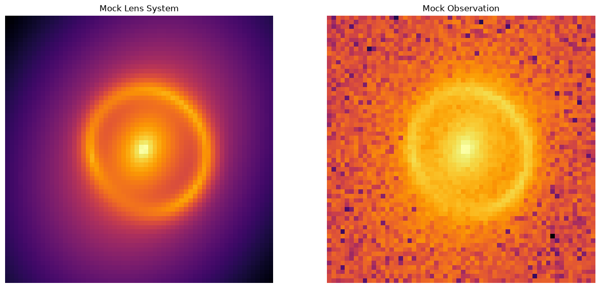
Here we write out the true values for all the parameters in the model. In total there are 21 parameters, so this is quite a complex model already! We then plot the data so we can see what it is we re trying to fit.
tensor([ 0.0500,  0.0000,  0.8600, -0.2000,  0.6600,  0.0000, -0.0500,  0.1000,
         0.0000,  0.7500,  1.1800,  1.0000,  0.1155,  0.0400,  0.0500,  0.0000,
         0.7500,  1.1800,  2.0000,  0.6928,  0.0400])
1.0110719129774306
Fit using emcee#
We now model the data using emcee which handles standard Metropolis-Hastings MCMC sampling (plus a few tricks). First we need to construct a log likelihood function. In our case this is just the squared residuals, divided by the variance in each pixel. The rest is specific to the emcee implementation. Note that we must use many walkers due to the algorithm emcee uses, since this is a 21 dimensional problem we need at least 42 chains and we use 64 since that is a nice power of 2.
# Make batched simulator
vsim = torch.vmap(sim)


# Log-likelihood function
def density(x):
    model = vsim(torch.as_tensor(x, dtype=torch.float32))
    log_likelihood_value = -0.5 * torch.sum(
        ((model - obs_system) ** 2) / variance, dim=(1, 2)
    )
    log_likelihood_value = torch.nan_to_num(log_likelihood_value, nan=-np.inf)
    return log_likelihood_value.numpy()


nwalkers = 64
ndim = len(true_params)

sampler = emcee.EnsembleSampler(nwalkers, ndim, density, vectorize=True)

x0 = true_params + 0.01 * torch.randn(nwalkers, ndim, dtype=torch.float32)
print("burn-in")
state = sampler.run_mcmc(x0, 100, skip_initial_state_check=True)  # burn-in
sampler.reset()
print("production")
state = sampler.run_mcmc(state, 1000)  # production
burn-in
production
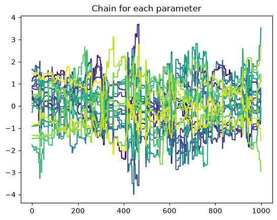
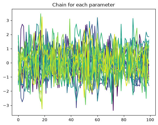
We have taken 64000 samples in this demo, in general you would want many more (each chain needs to run longer than 1000 steps in order to fully mix). Its always a good idea to plot the chains and check that they don’t have any pathological features (i.e. getting frozen at one value). We subtract the mean and divide by the standard deviation of each parameter so that the chains can all be plotted together despite having very different values. Here we can see the non zero autocorrelation length for one of the chains even over 1000 steps. This indicates we should run the chains much longer, but this is just a demo.
chain_mh = sampler.get_chain()
normed_chains = (chain_mh[:, 0] - np.mean(chain_mh[:, 0], axis=0)) / np.std(
    chain_mh[:, 0], axis=0
)
for i in range(chain_mh.shape[2]):
    plt.plot(normed_chains[:, i], color=colormaps["viridis"](i / chain_mh.shape[2]))
plt.title("Chain for each parameter")
plt.show()
Since the autocorrelation length is >1, we can compute an effective sample size to determine how many equivalent independent points we have drawn. As the warning suggests, in this demo we cannot compute the actual autocorrelation length, the autocorrelation length increases as we draw more samples (you can test this by changing the 1000 above to a larger number). Assuming that the autocorrelation is actually of a similar length to the chain (1000), this means we have drawn approximately 64 independent samples (one for each walker).
print(
    "Autocorrelation time: ",
    np.mean(emcee.autocorr.integrated_time(chain_mh, quiet=True)),
)
The chain is shorter than 50 times the integrated autocorrelation time for 21 parameter(s). Use this estimate with caution and run a longer chain!
N/50 = 20;
tau: [ 89.72725685  99.53533102  78.00108107 109.95159024  77.80314436
  89.22623745  95.72411722  81.96200771  82.88745681  88.69844611
  82.93342122  97.33354396  93.77565257  91.70370788  71.16883732
  79.53494194  93.7727209   80.77516954 121.97110636  93.43388245
 112.04880852]
Autocorrelation time: 91.04611721453405
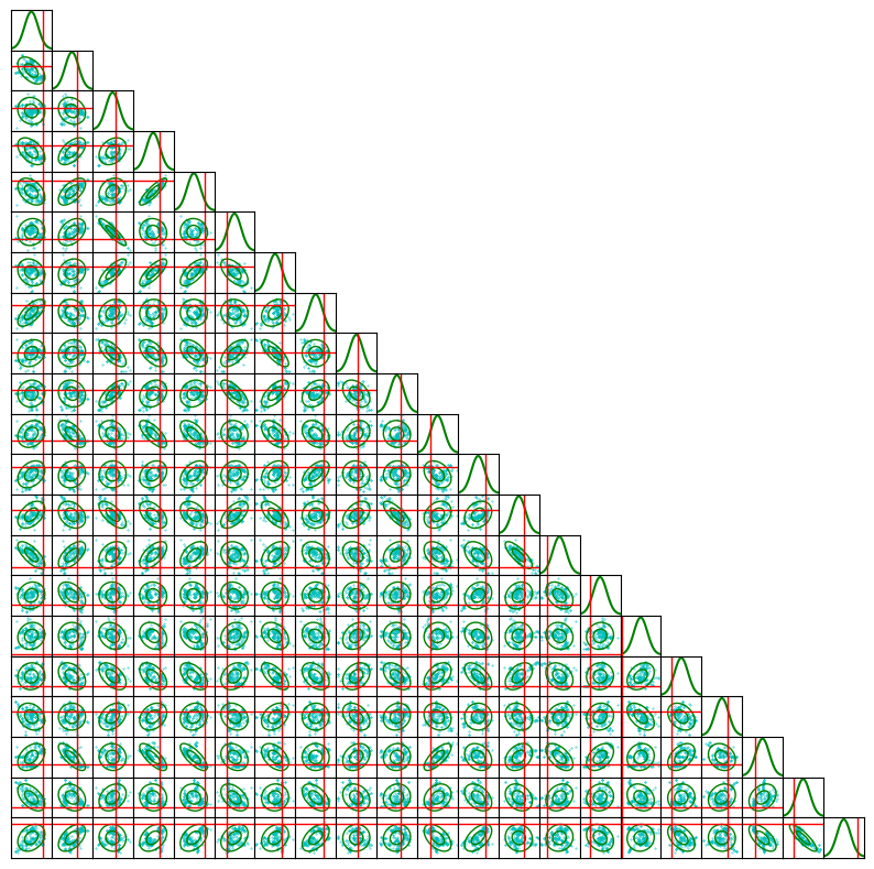
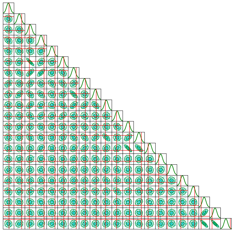
We may plot the samples in a corner plot. However, we thin the samples first so that the number of points is not overwhelming to plot. As you can see in the subfigures there is still a bloby structure of the samples, suggesting that the chains were not run long enough to converge and fill the probability volume.
In this figure the green contours show the covariance matrix computed from the samples, the cyan points are the samples themselves, and the red lines are ground truth.
N = chain_mh.shape[0] * chain_mh.shape[1]
fig = corner_plot(
    np.concatenate(chain_mh, axis=0)[:: int(N / 200)],
    true_values=true_params.numpy(),
)
plt.show()
Fit with MALA sampling#
Metropolis Adjusted Langevin Algorithm (MALA) sampling is the half way point between NUTS and MH, it uses gradient information to make an efficient proposal distribution for a MH step. We have written a basic implementation below for demo purposes. Essentially, one uses a random perturbation like in MH, except with a bias towards higher likelihood which comes from the gradient. Detailed balance is maintained using a MH step, so we still sample the correct distribution.
def mala_sampler(
    initial_state,  # (num_chains, D)
    log_prob,  # x -> (num_chains,)
    log_prob_grad,  # x -> (num_chains, D)
    num_samples,
    epsilon,
    mass_matrix,  # covariance
    progress=True,
    desc="MALA",
):
    x = np.array(initial_state, copy=True)
    C, D = x.shape

    # mass, inv_mass, L
    mass = np.array(mass_matrix, copy=False)  # (D, D)
    inv_mass = np.linalg.inv(mass)  # (D, D)
    L = np.linalg.cholesky(mass)  # (D, D)

    samples = np.zeros((num_samples, C, D), dtype=x.dtype)  # (N, C, D)

    # Cache current state
    logp_cur = log_prob(x)  # (C,)
    grad_cur = log_prob_grad(x)  # (C, D)

    # Random number generator
    rng = np.random.default_rng(np.random.randint(1e10))

    it = range(num_samples)
    if progress:
        it = tqdm(it, desc=desc, position=0, leave=True)

    for t in it:
        # proposal using current grad
        mu_x = 0.5 * (epsilon**2) * (grad_cur @ mass)  # (C, D)
        noise = rng.standard_normal((C, D)) @ L.T  # (C, D)
        x_prop = x + mu_x + epsilon * noise  # (C, D)

        # Evaluate proposal
        logp_prop = log_prob(x_prop)  # (C,)
        grad_prop = log_prob_grad(x_prop)  # (C, D)

        mu_xprop = 0.5 * (epsilon**2) * (grad_prop @ mass)  # (C, D)

        # q(x|x') \propto \exp(-0.5|x - x' - mu(x')|^2 / \epsilon^2)
        d1 = x - x_prop - mu_xprop  # for q(x | x')
        d2 = x_prop - x - mu_x  # for q(x'| x)

        logq1 = -0.5 * np.einsum("bi,ij,bj->b", d1, inv_mass, d1) / epsilon**2  # (C,)
        logq2 = -0.5 * np.einsum("bi,ij,bj->b", d2, inv_mass, d2) / epsilon**2  # (C,)

        log_alpha = (logp_prop - logp_cur) + (logq1 - logq2)  # (C,)

        accept = np.log(rng.random(C)) < log_alpha  # (C,)

        # Update all three pieces in-place where accepted
        x[accept] = x_prop[accept]  # (C, D)
        logp_cur[accept] = logp_prop[accept]  # (C,)
        grad_cur[accept] = grad_prop[accept]  # (C, D)

        samples[t] = x

        if progress:
            it.set_postfix(acc_rate=f"{accept.mean():0.2f}")

    return samples
Here we run the MALA sampler after a small burn-in. We cheat a little bit and use the previous sampler to construct a mass matrix, this makes MALA more efficient but you could just as easily set the mass matrix to identity for the burn-in then use the burn-in samples to get a mass matrix, it only requires more fiddling with parameters (epsilon).
def density_grad(x):
    x = torch.as_tensor(x, dtype=torch.float32)
    x.requires_grad = True
    model = vsim(x)
    log_likelihood_value = -0.5 * torch.sum(
        ((model - obs_system) ** 2) / variance, dim=(1, 2)
    )
    log_likelihood_value = torch.nan_to_num(log_likelihood_value, nan=-np.inf)
    log_likelihood_value.sum().backward()
    return x.grad.numpy()


nwalkers = 32
x0 = true_params + 0.01 * torch.randn(nwalkers, ndim, dtype=torch.float32)
cov = np.cov(chain_mh.reshape(-1, ndim), rowvar=False)
# cov = np.linalg.inv(np.cov(chain_mh.reshape(-1, ndim), rowvar=False))

chain_burnin_mala = mala_sampler(
    initial_state=x0,
    log_prob=density,
    log_prob_grad=density_grad,
    num_samples=100,
    epsilon=3e-1,
    mass_matrix=cov,
    desc="Warmup",
)  # burn-in

chain_mala = mala_sampler(
    initial_state=chain_burnin_mala[-1],
    log_prob=density,
    log_prob_grad=density_grad,
    num_samples=1000,
    epsilon=7e-1,
    mass_matrix=cov,
    desc="Production",
)  # production
/tmp/ipykernel_1158/3428914965.py:11: DeprecationWarning: __array__ implementation doesn't accept a copy keyword, so passing copy=False failed. __array__ must implement 'dtype' and 'copy' keyword arguments. To learn more, see the migration guide https://numpy.org/devdocs/numpy_2_0_migration_guide.html#adapting-to-changes-in-the-copy-keyword
  x = np.array(initial_state, copy=True)
Plotting the chains we see that they mix much better than the MH sampler, but still have some autocorrelation, as would be expected.
The autocorrelation length is better than MH as expected. Again the effective sample size can’t be trusted and is probably a bit larger than the 64 value from before.
print(
    "Autocorrelation time: ",
    np.mean(emcee.autocorr.integrated_time(chain_mala, quiet=True)),
)
The chain is shorter than 50 times the integrated autocorrelation time for 12 parameter(s). Use this estimate with caution and run a longer chain!
N/50 = 20;
tau: [15.29095728 12.57274965 21.21580997 32.13391978 13.56800966 19.16705842
 28.05291087 13.17535197 21.35735972 26.94996406 21.55044702 43.1721109
 39.44951084 41.87775682  8.70514168  9.15876818 15.85068825 18.81650515
 35.69698881 33.58678402 34.93598515]
Autocorrelation time: 24.108798962241963
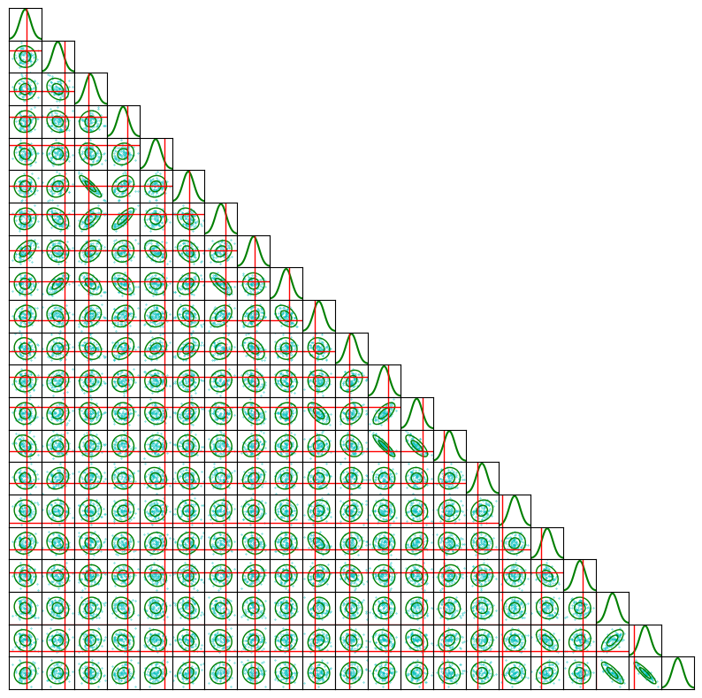
The corner plot is much better than the MH example, we can see how the volume is filled out more with fewer gaps, suggesting we have sampled a good chunk of the space.
Fit using NUTS#
We now model the data using NUTS. A prior is required, so we just set some extremely wide values so that we will explore just the likelihood; in general one would want to pick more informative priors. The rest is specific to the Pyro NUTS implementation!
Note, we use 25 warmup steps for Pyro, this is so it can automatically determine an appropriate “mass matrix” which helps the sampler explore much more efficiently! NUTS can also determine its own step size and build a full mass matrix. For a real analysis you would likely want to take many warm up steps so it can figure these things out accurately, afterwards the sampling will be incredibly efficient. For the sake of time in this demo, we preset a bunch of parameters and restrict what it can do, we will still get quite excellent samples.
def step(model, prior):
    x = pyro.sample("x", prior)
    # Log-likelihood function
    res = model(x)
    log_likelihood_value = -0.5 * torch.sum(((res - obs_system) ** 2) / variance)
    # Observe the log-likelihood
    pyro.factor("obs", log_likelihood_value)


prior = dist.Normal(
    true_params,
    torch.ones_like(true_params) * 1e2 + torch.abs(true_params) * 1e2,
)
nuts_kwargs = {
    "jit_compile": True,
    "ignore_jit_warnings": True,
    "step_size": 2e-2,
    "full_mass": False,
    "adapt_step_size": False,
    "adapt_mass_matrix": True,
    "target_accept_prob": 0.8,
    "max_tree_depth": 8,
}

nuts_kernel = pyro_NUTS(step, **nuts_kwargs)
init_params = {"x": true_params.clone()}

# Run MCMC with the NUTS sampler and the initial guess
mcmc_kwargs = {
    "num_samples": 100,
    "warmup_steps": 25,
    "initial_params": init_params,
    "disable_progbar": False,
}

mcmc = pyro_MCMC(nuts_kernel, **mcmc_kwargs)

mcmc.run(sim, prior)
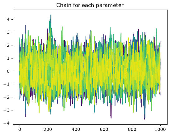
We have only taken 100 samples in this demo, in general you would want many more. Again we plot the chains and check that they look uncorrelated, everything seems fine here! There is much less structure than before, it looks like we are sampling random noise which is ideal.
chain_nuts = mcmc.get_samples()["x"]
chain_nuts = chain_nuts.numpy()

normed_chains = (chain_nuts - np.mean(chain_nuts, axis=0)) / np.std(chain_nuts, axis=0)
for i in range(chain_nuts.shape[1]):
    plt.plot(normed_chains[:, i], color=colormaps["viridis"](i / chain_nuts.shape[1]))
plt.title("Chain for each parameter")
plt.show()

print(
    "Autocorrelation time: ",
    np.mean(
        emcee.autocorr.integrated_time(
            chain_nuts, has_walkers=False, tol=10, quiet=True
        )
    ),
)
Autocorrelation time: 1.7549979950112866
As is common for NUTS sampling, the average autocorrelation time for the parameters is around 1, meaning that essentially every sample is independent.
Finally, we show the corner plot where the samples are very well distributed as we would expect for uncorrelated samples.
fig = corner_plot(chain_nuts, true_values=true_params.numpy())
plt.show()
The Pyro NUTS implementation is very convenient in that it handles the tuning of all parameters automatically in the warmup phase. In practice however, the small but efficient steps of MALA often make it very efficient, plus the rapid progress makes it easier to tweak and tune the sampler to your problem. Emcee will struggle with high dimensional problems, it was already having a hard time at 21 dimensions and gravitational lensing analysis can go much beyond 21 parameters, but it doesn’t require gradient computations which may be impractical for some forward models. In the end, your specific problem will likely determine which algorithm to use.