Let’s take a deeper dive into Caustics!

Let’s take a deeper dive into Caustics!#

In this introduction, we will showcase some of the features and design principles of caustics. We will see

How to get started from one of our pre-built Simulator
Visualization of the Simulator graph (DAG of caustics modules)
Distinction between Static and Dynamic parameters
How to create a a batch of simulations
Semantic structure of the Simulator input
Taking gradient w.r.t. to parameters with Pytorch autodiff functionalities
Swapping in flexible modules like the Pixelated representation for more advanced usage
How to create your own Simulator

Getting started with the `LensSource` Simulator#

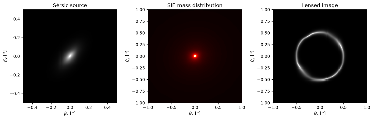
For this first introduction, we use the simplest modules in caustics for the lens and source, namely the SIE and the Sersic modules. We also assume a FlatLambdaCDM cosmology.

from caustics import LensSource, SIE, Sersic, FlatLambdaCDM

# Define parameters of the camera pixel grid
pixelscale = 0.04  # arcsec/pixel
pixels = 100

# Instantiate modules for the simulator
cosmo = FlatLambdaCDM(name="cosmology")
lens = SIE(
    cosmology=cosmo, name="lens", z_s=1, z_l=0.5, x0=0, y0=0, q=0.9, phi=0.4, Rein=1
)
source = Sersic(name="source", x0=0, y0=0, q=0.5, phi=0.9, n=1, Re=0.1, Ie=10)
simulator = LensSource(lens, source, pixelscale=pixelscale, pixels_x=pixels)

Generating a simulation of a strong gravitational lens#

# Generate a lensed image
y = simulator(params=params)

Text(0.5, 0, "$\\theta_x$ ['']")

../_images/32a09a25c70d848d62369fd818876676591b4f1225356f56e3e56e041f54bef4.png

Visualization of the `Simulator` DAG#

simulator.graphviz()

../_images/47be82097bf589dae091a61059abe2782a913a97ed3ac440a877b2977adb1414.svg

Static vs Dynamic parameters#

In the DAG shown above,

Dynamic parameters are shown in white boxes
Static parameters are shown in grey boxes

The distinction between the two types can be summarized as follows

Dynamic parameters are fed as input to the simulator and can be batched over (data parallelism)
Static parameters have fixed values. Their values is stored in the internal DAG, and will be broadcasted over when batching computation

# Making a parameter dynamic
simulator.lens.z_s.to_dynamic()
simulator.graphviz()  # z_s turns white, which makes it disappear when we don't show the dynamic parameters (first option False)

../_images/68c2a2fb70b459888024c59b9c12ecfcfd431aae2ecf6c2afc90b42aac23a9ab.svg

# Making a parameter static
simulator.lens.z_s.to_static()
simulator.graphviz()  # z_s turns grey

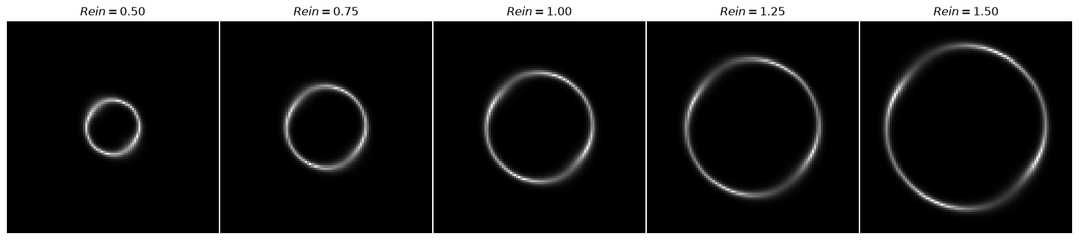
Simulating a batch of observations#

We use vmap over the simulator to create a batch of parameters. In this example, we create a batch of examples that only differ by their Einstein radius. To do this, we turn all the other parameter into static parameters. This is done in the hidden cell below

# Create a grid of Einstein radius
b = torch.linspace(0.5, 1.5, 5).view(-1, 1)  # Shape is [B, 1]
ys = vmap(simulator)(b)

../_images/356c72a3c5f7ef06b19f88ddf390ede615d99f153b4b934b077921cafa16fbf0.png

Semantic structure of the input#

The simulator’s input takes different format to allow different usecase scenarios

Flattened tensor for deep neural network like in Hezaveh et al. (2017)
Semantic List to separate the input int terms of high level modules like Lens and Source
Low-level Dictionary to decompose the parameters at the level of the leafs of the DAG

Below, we illustrate how to use all of these structures. For completeness, we also use vmap.

# Make some parameters dynamic for this example
simulator.source.Ie.to_dynamic()
simulator.lens.Rein.to_dynamic()

Flattened Tensor#

To make sure the order of the parameter is correct, print the simulator. Order of dynamic parameters is read top to bottom.

print(simulator)

sim|LensSource
    psf|static: 1
    x0|static: 0
    y0|static: 0
    lens|SIE
        cosmology|FlatLambdaCDM
            h0|static: 0.677
            critical_density_0|static: 1.27e+11
            Om0|static: 0.31
        z_s|static: 1
        z_l|static: 0.5
        x0|static: 0
        y0|static: 0
        q|static: 0.9
        phi|static: 0.4
        Rein|dynamic: 1
    source|Sersic
        x0|static: 0
        y0|static: 0
        q|static: 0.5
        phi|static: 0.9
        n|static: 1
        Re|static: 0.1
        Ie|dynamic: 10

B = 5  # Batch dimension
Rein = torch.rand(B, 1)
Ie = torch.rand(B, 1)
x = torch.concat([Rein, Ie], dim=1)  # Concat along the feature dimension

# Now we can use vmap to simulate multiple images at once
ys = vmap(simulator)(x)

Semantic lists#

A semantic list is simply a list over module parameters like the one we used earlier: [lens_params, source_params]. Note that we could also include cosmological parameters in that list

B = 5
cosmo_param = torch.rand(B, 1)  # h0
lens_x0_param = torch.randn(B, 1)  # x0
lens_Rein_param = torch.randn(B, 1)  # Rein
source_param = torch.rand(B, 1)  # Ie

x = torch.cat([cosmo_param, lens_x0_param, lens_Rein_param, source_param], dim=-1)
ys = vmap(simulator)(x)

Low-level Dictionary#

Make the dictionary have the same structure as the graph.

x = {
    "lens": {
        "x0": x0,
        "Rein": Rein,
        "cosmology": {
            "h0": h0,
        },
    },
    "source": {
        "Ie": Ie,
    },
}
ys = vmap(simulator)(x)

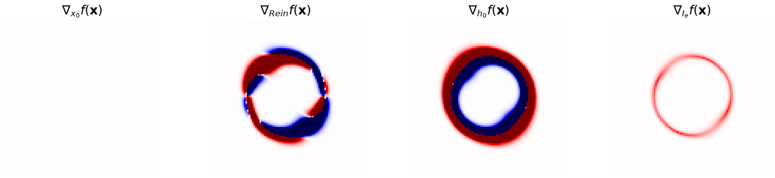
Computing gradients with automatic differentiation#

Computing gradients is particularly useful for optimization. Since taking gradients w.r.t. list or dictionary inputs is not possible with torch.func.grad, we will need a small wrapper around the simulator. For optimisation, the wrapper will often be a log likelihood function. For now we use a generic lambda wrapper.

In the case of the semantic list input, the wrapper has the general form

lambda *x: simulator(x)

The low-level dictionary input is a bit more involved but can be worked out on a case by case basis.

Note: apply vmap around the gradient function (e.g. jacfwd or grad) to handle batched computation

jacfwd will return a list of 3 tensors of shape [B, pixels, pixels, D], where D is the number of parameters in that module

jac = jacfwd(lambda *x: simulator(x), argnums=(0, 1, 2, 3))(
    cosmo_param, lens_x0_param, lens_Rein_param, source_param
)

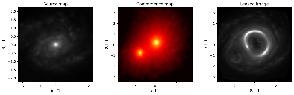
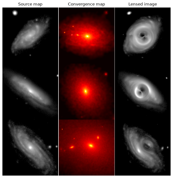
../_images/959197b4fc5f7e151afffaa988afe6f7a4bc3c36d919432e8cd0c842465c023b.png

Pixelated representations#

The examples above made use of very simplistic modules. Here, we will showcase how easily we can swap-in flexible representations to represent more realistic systems.

Pixelated is the module used to represent the background source with a grid of pixels
PixelatedConvergence is the module used to represent the convergence of the lens with a grid of pixels

For this example, we will use source samples from the PROBES dataset (Stone et al., 2019) and convergence maps sampled from Illustris TNG (Nelson et al., 2019, see Adam et al., 2023 for preprocessing, or use this link to download the maps).

from caustics import Pixelated, PixelatedConvergence

# Some static parameters for the simulator
pixelscale = 0.07
source_pixelscale = 0.25 * pixelscale
z_l = 0.5
z_s = 1.0
x0 = 0
y0 = 0

# Construct the Simulator with Pixelated and PixalatedConvergence modules
cosmo = FlatLambdaCDM(name="cosmo")
source = Pixelated(
    name="source", shape=(256, 256), pixelscale=source_pixelscale, x0=x0, y0=y0
)
lens = PixelatedConvergence(
    cosmology=cosmo,
    name="lens",
    pixelscale=pixelscale,
    shape=(128, 128),
    z_l=z_l,
    z_s=z_s,
)
simulator = LensSource(lens, source, pixelscale=pixelscale, pixels_x=pixels)

simulator.graphviz()

../_images/bc8b620549bda94abd956a0b2ae1e9e5876c924ce60d9c3611e3fde86d40c186.svg

In the hidden cell below, we load the maps from a dataset. If you downloaded the datasets mentioned above, you can use the code below to load maps from them.

Make a simulation by feeding the maps as input to the simulator (using semantic list inputs)

y = simulator([kappa_map, source_map])

Text(0.5, 1.0, 'Lensed image')

../_images/a12f1d574d3477524b6bb46923852b38bd9736fd87c0b0abfbd25ab2e7b704c9.png

Of course, batching works the same way as before and is super fast. Below, we show the time it takes to make 4 batched simulations on a laptop.

%%timeit

ys = vmap(simulator)([kappa_maps, source_maps])

13.2 ms ± 293 μs per loop (mean ± std. dev. of 7 runs, 100 loops each)

../_images/d5b05d04cb1108a3b712a53de23693337f4d6ec3ed05b95d0c97582efe369931.png

Creating your own Simulator#

Here, we only introduce the general design principles to create a simulator. More comprehensive explanations can be found in the caskade docs.

A Simulator is very much like a neural network in Pytorch#

A simulator inherits from the super class caskade.Module, similar to how a neural network inherits from the nn.Module class in Pytorch

from caustics import Module, Param, forward

class MySim(Module):
    def __init__(self):
        super().__init__()
        self.p = Param("p")

    @forward
    def myfunction(self, x, p):
        ...

The init method constructs the computation graph, initialize the caustics modules, and can prepare or store variables for the forward method.
The forward method is where the actual simulation happens.
x generally denotes a set of parameters which affect the computations in the simulator graph.

How to use a Simulator in your workflow#

Like a neural network, MySim (and in general any caustics modules), must be instantiated outside the main workload. This is because caustics builds a graph internally every time a module is created. Ideally, this happens only once to avoid overhead. In general, you can follow the following code pattern

# Instantiation
simulator = MySim()

# Heavy workload
for n in range(N):
    y = vmap(simulator)(x)

This allows you to perform inefficient computations that only need to happen once in the __init__ method while keeping your forward method lightweight.

How to feed parameters to the different modules#

This is probably the easiest part of building a Simulator, you only provide the values when calling the top level simulator.

Here is a minimal example that shows how to feed the parameters the forward method

@forward
def raytrace(self, x, y):
   alpha_x, alpha_y = self.lens.reduced_deflection_angle(x, y)
   beta_x = x - alpha_x # lens equation
   beta_y = y - alpha_y
   return self.source.brightness(beta_x, beta_y)
sim.raytrace(xgrid, ygrid, params)

You might worry that params can have a relatively complex structure (flattened tensor, semantic list, low-level dictionary). caustics handles this complexity for you. You only need to make sure that params contains all the dynamic parameters required by your custom simulator. This design works for every caustics module and each of their methods, meaning that params is always the last argument in a caustics method call signature.

The only details that you need to handle explicitly in your own simulator are stuff like the camera pixel position (xgrid and ygrid), and source redshifts (z_s). Those are often constructed in the __init__ method because they can be assumed fixed. Thus, the example above assumed that they can be retrieved from the self registry. A Simulator is often an abstraction of an instrument with many fixed variables to describe it, or aimed at a specific observation.

Of course, you could have more complex workflows for which this assumption is not true. For example, you might want to infer the PSF parameters of your instrument and need to feed this to the simulator as a dynamic parameter. The next section has what you need to customize completely your simulator

Creating your own variables as leafs in the DAG#

You can register new variables in the DAG for custom calculations as follows

from caustics import Module, forward, Param


class MySim(Module):
    def __init__(self):
        super().__init__()  # Don't forget to use super!!
        # shape has to be a tuple, e.g. shape=(1,). This can be any shape you need.
        self.my_dynamic_arg = Param(
            "my_dynamic_arg", value=None, shape=(1,)
        )  # register a dynamic parameter in the DAG
        self.my_static_arg = Param(
            "my_static_arg", value=1.0, shape=()
        )  # register a static parameter in the DAG

    @forward
    def forward(self, x, my_dynamic_arg, my_static_arg):

        # My very complex workflow
        ...
        return my_dynamic_arg * x + my_static_arg


sim = MySim()
sim.graphviz()

../_images/2dd77f65ae66d5a751c0a146014cf75a1f90c5223ae53896f5875ef94636d47c.svg