Making a new lens model

Making a new lens model#

Here we will demo how you can make your own lens model just by defining a potential, caustics will take care of the rest.

%load_ext autoreload
%autoreload 2
%matplotlib inline

import matplotlib.pyplot as plt
import torch
import caustics
from caustics import forward, Param

Below we define a class that inherits from caustics.ThinLens, this is the abstract class for all single plane lenses in caustics. The base class needs a cosmology, lens redshift, and source redshift which are passed via super(). After that we define the Params needed by our class (which is just some gaussian parameters). Finally, we define the potential function for our class, which in this case is a gaussian. The potential is convenient because all other lensing quantities (deflection angle and convergence) can be determined from derivatives of the potential. This is why, given only the potential, caustics is able to build a full model.

class GaussianPotential(caustics.ThinLens):

    def __init__(self, cosmology, z_l, z_s, x0, y0, A, sigma):
        super().__init__(cosmology=cosmology, z_l=z_l, z_s=z_s)

        self.x0 = Param("x0", x0)
        self.y0 = Param("y0", y0)
        self.A = Param("A", A)
        self.sigma = Param("sigma", sigma)

    @forward
    def potential(self, x, y, x0, y0, A, sigma):
        return -A * torch.exp(-((x - x0) ** 2 + (y - y0) ** 2) / (2 * sigma**2))

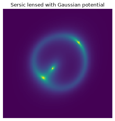
Now we can do a really basic simulation just to see everything is working. We take a Sersic source model and use the LensSource simulator to make an image of the lensing from our gaussian potential model.

cosmo = caustics.FlatLambdaCDM()
lens = GaussianPotential(cosmo, z_l=0.5, z_s=1.0, x0=0.0, y0=0.0, A=2.0, sigma=1.0)
src = caustics.Sersic(x0=0.2, y0=0.2, q=0.6, phi=1.0, Ie=1.0, Re=1.0, n=2.0)

sim = caustics.LensSource(lens, src, pixels_x=100, pixelscale=0.05, upsample_factor=2)

plt.imshow(sim().numpy(), origin="lower")
plt.axis("off")
plt.title("Sersic lensed with Gaussian potential")
plt.show()

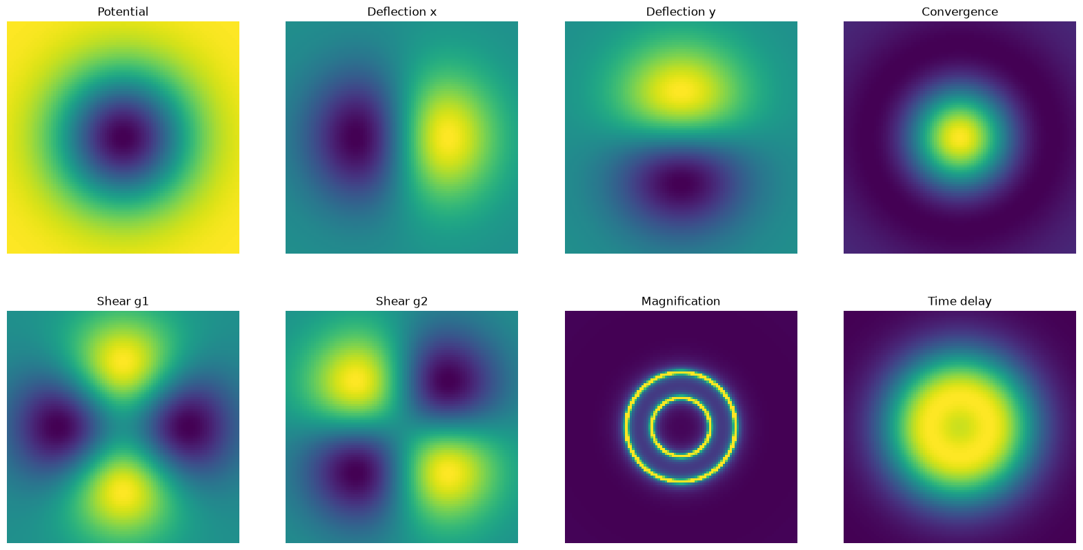
../_images/2fc2a84833c44bc61bc0790c045d5e141a71980b2309b549ede5b985eacd1424.png

Now that we’ve tried lensing, lets look at all the basic lensing quantities and map them out for our new lens. The potential is exactly as we specified, the deflection angles are its derivatives, the convergence comes from second derivatives, and so on. We can compute shear, magnification, and the time delay field as well.

(np.float64(-0.5), np.float64(99.5), np.float64(-0.5), np.float64(99.5))

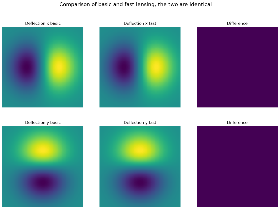
../_images/d0ca845afab9f70b01bc14810a328ba4ba8e29c10e5b7ab019705add360c3165.png

If you know the analytic form of one of the quantities, you may want to write out the appropriate function and overload the base class method which uses autograd to compute it. This will be faster since you’ve done some of the work for the code by figuring out the analytic form.

class GaussianPotentialFast(caustics.ThinLens):

    def __init__(self, cosmology, z_l, z_s, x0, y0, A, sigma):
        super().__init__(cosmology=cosmology, z_l=z_l, z_s=z_s)

        self.x0 = Param("x0", x0)
        self.y0 = Param("y0", y0)
        self.A = Param("A", A)
        self.sigma = Param("sigma", sigma)

    @forward
    def potential(self, x, y, x0, y0, A, sigma):
        return -A * torch.exp(-((x - x0) ** 2 + (y - y0) ** 2) / (2 * sigma**2))

    @forward
    def reduced_deflection_angle(self, x, y, x0, y0, A, sigma):
        ax = -(x - x0) / sigma**2  # derivative of exponent
        ay = -(y - y0) / sigma**2
        p = self.potential(x, y)  # exponential stays after derivative
        return ax * p, ay * p

    @forward
    def convergence(self, x, y, x0, y0, A, sigma):
        p = self.potential(x, y)
        dx = (x - x0) ** 2 / sigma**4
        dxdx = -1 / sigma**2
        dy = (y - y0) ** 2 / sigma**4
        return 0.5 * (2 * dxdx + dx + dy) * p

../_images/c0a9da90c3542046c78020ee649186bd47813db8b94e2a93657c8cc1d81f8d16.png

%%timeit
ax, ay = lens_basic.reduced_deflection_angle(thx, thy)

751 μs ± 2.31 μs per loop (mean ± std. dev. of 7 runs, 1,000 loops each)

%%timeit
ax, ay = lens_fast.reduced_deflection_angle(thx, thy)

159 μs ± 558 ns per loop (mean ± std. dev. of 7 runs, 10,000 loops each)

Here we see that our new fast version is much faster (almost 10x faster) than the basic one which only uses automatic differentiation from the potential. There are a few reasons for this, in the most straightforward setups it is normal for autograd to be about 2-3x slower than an analytic derivation. Further, because in this case there are many shared calculations between ax and ay, we were able to save ourselves a bunch of calculations by only doing the shared stuff once.

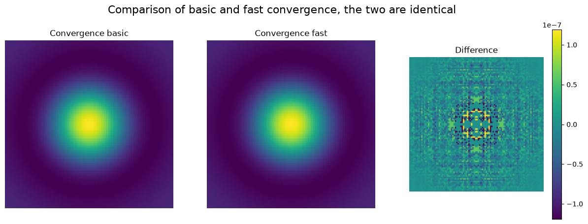
Next lets look at the convergence, which uses the Hessian of the potential. Below we compare the two ways of computing the convergence, one using autograd and the other using analytic derivatives. We see that the two are nearly identical, the residuals are at the level of 10^-7 which is the precision of floating point operations. Thus the two are identical up to the level that we can tell with our current numerical precision.

../_images/a02bd47e8c2e0790132173da8c886356cff8d19c10a0fdba55d117e8d1447182.png

%%timeit
kappa = lens_basic.convergence(thx, thy)

5.13 ms ± 30.8 μs per loop (mean ± std. dev. of 7 runs, 100 loops each)

%%timeit
kappa = lens_fast.convergence(thx, thy)

191 μs ± 1.49 μs per loop (mean ± std. dev. of 7 runs, 10,000 loops each)

Since the convergence uses second derivatives, we see an even more dramatic difference between our basic autograd from the potential and an analytic calculation. It is now almost 30x faster, which is another factor of 3 because of the extra autograd operation needed for the basic calculation.

The conclusion here is that using autograd from the potential is easy and reasonably fast, but if performance is a significant value then its worth doing the extra work to get the derivatives yourself. In caustics all of the base models have analytic potential, deflection_angle, and convergence so that it is as performant as possible. If you can use a built-in method of caustics then it is worth doing so, but if you need to make your own model, you now know how to make it as fast as possible!