Inverting the Lens Equation

The lens equation \(\vec{\beta} = \vec{\theta} - \vec{\alpha}(\vec{\theta})\) allows us to find a point in the source plane given a point in the image plane. However, sometimes we know a point in the source plane and would like to see where it ends up in the image plane. This is not easy to do since a point in the source plane may map to multiple locations in the image plane. There is no closed form function to invert the lens equation, in large part because the deflection angle \(\vec{\alpha}\) depends on the position in the image plane \(\vec{\theta}\). To invert the lens equation, we will need to rely on optimization and a iterative procedures to find all the images for a given source plane point. Below we will demonstrate how this is done in caustics!

%load_ext autoreload
%autoreload 2


import torch
import matplotlib.pyplot as plt
from matplotlib.patches import Polygon
from matplotlib.collections import PatchCollection
import numpy as np

import caustics

# initialization stuff for an SIE lens

cosmology = caustics.FlatLambdaCDM(name="cosmo")
cosmology.to(dtype=torch.float32)
n_pix = 100
res = 0.05
upsample_factor = 1
fov = res * n_pix
thx, thy = caustics.utils.meshgrid(
    res / upsample_factor,
    upsample_factor * n_pix,
    upsample_factor * n_pix,
    dtype=torch.float32,
)
z_l = torch.tensor(0.5, dtype=torch.float32)
z_s = torch.tensor(1.5, dtype=torch.float32)
lens = caustics.SIE(
    cosmology=cosmology,
    name="sie",
    z_l=z_l,
    z_s=z_s,
    x0=0.0,
    y0=0.0,
    q=0.4,
    phi=np.pi / 5,
    Rein=1.0,
    s=1e-3,
)

Here we run the forward raytracing for our particular lens model. In caustics we provide a convenient forward_raytrace function which can be called for any lens model. Internally, this constructs a number of triangles in the image plane, raytraces them to the source plane and identifies which ones contain the desired source plane position. Iteratively subdividing the triangles eventually converges on image plane positions which map to the desired source plane position. See further down for more detail.

# Point in the source plane
sp_x = torch.tensor(0.2)
sp_y = torch.tensor(0.2)

# Points in image plane
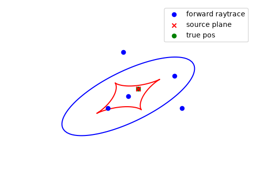
x, y = lens.forward_raytrace(sp_x, sp_y)

# Raytrace to check
bx, by = lens.raytrace(x, y)

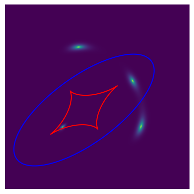
When we raytrace the coordinates we get out from forward_raytrace it is not too surprising that they all give source plane positions very close to the desired source plane position. Here we plot them so you can see:

Show code cell source

Hide code cell source

fig, ax = plt.subplots()

A = lens.jacobian_lens_equation(thx, thy)
detA = torch.linalg.det(A)

CS = ax.contour(thx, thy, detA, levels=[0.0], colors="b", zorder=1)
# Get the path from the matplotlib contour plot of the critical line
paths = CS.allsegs[0]
caustic_paths = []
for path in paths:
    # Collect the path into a discrete set of points
    x1 = torch.tensor(list(float(vs[0]) for vs in path))
    x2 = torch.tensor(list(float(vs[1]) for vs in path))
    # raytrace the points to the source plane
    y1, y2 = lens.raytrace(x1, x2)

    # Plot the caustic
    ax.plot(y1, y2, color="r", zorder=1)
ax.scatter(x, y, color="b", label="forward raytrace", zorder=10)
ax.scatter(bx, by, color="r", marker="x", label="source plane", zorder=9)
ax.scatter([sp_x.item()], [sp_y.item()], color="g", label="true pos", zorder=8)
ax.set_axis_off()
plt.legend()
plt.show()

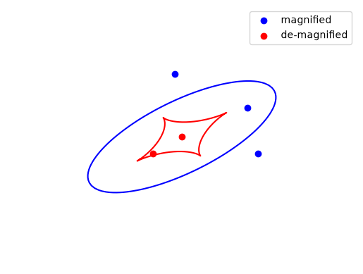
It is also often not necessary to model the central demagnified region since it is so faint (approximately a 100,000 times fainter in this case) that it doesn’t contribute measurably to the flux of an image. We can very easily check the magnification of every point and remove the unnecessary one.

m = lens.magnification(x, y)
print(m.detach().cpu().tolist())

fig, ax = plt.subplots()
CS = ax.contour(thx, thy, detA, levels=[0.0], colors="b", zorder=1)
# Get the path from the matplotlib contour plot of the critical line
for path in paths:
    # Collect the path into a discrete set of points
    x1 = torch.tensor(list(float(vs[0]) for vs in path))
    x2 = torch.tensor(list(float(vs[1]) for vs in path))
    # raytrace the points to the source plane
    y1, y2 = lens.raytrace(x1, x2)

    # Plot the caustic
    ax.plot(y1, y2, color="r", zorder=1)

plt.scatter(x[m >= 1], y[m >= 1], color="b", label="magnified")
plt.scatter(x[m < 1], y[m < 1], color="r", label="de-magnified")
plt.axis("off")
plt.legend()
plt.show()

[3.235136605204109e-06, 0.49296055603411754, 2.484502423396006, 2.2856878363623525, 3.1024166659768713]

Lets take a look

Using the LensSource simulator and the forward raytracing coordinates we can focus our calculations on the regions of interest for each image. Note however that the regions can overlap, which they do very slightly in this case.

src = caustics.Sersic(
    x0=0.2, y0=0.2, q=0.9, phi=0.0, n=1.0, Re=0.05, Ie=1.0, name="source"
)

sim = caustics.LensSource(
    lens=lens, source=src, x0=None, y0=None, pixelscale=0.005, pixels_x=100
)

# Plot the source and lens
fig, ax = plt.subplots()
CS = ax.contour(thx, thy, detA, levels=[0.0], colors="b", zorder=1)
# Get the path from the matplotlib contour plot of the critical line
for path in paths:
    # Collect the path into a discrete set of points
    x1 = torch.tensor(list(float(vs[0]) for vs in path))
    x2 = torch.tensor(list(float(vs[1]) for vs in path))
    # raytrace the points to the source plane
    y1, y2 = lens.raytrace(x1, x2)

    # Plot the caustic
    ax.plot(y1, y2, color="r", zorder=1)
for i in range(len(x)):
    ax.imshow(
        sim([x[i], y[i]]),
        extent=(
            -sim.pixelscale * sim.pixels_x / 2 + x[i],
            sim.pixelscale * sim.pixels_x / 2 + x[i],
            -sim.pixelscale * sim.pixels_y / 2 + y[i],
            sim.pixelscale * sim.pixels_y / 2 + y[i],
        ),
        origin="lower",
    )
ax.set_xlim([-1.5, 2])
ax.set_ylim([-1.5, 2])
ax.set_axis_off()
plt.show()

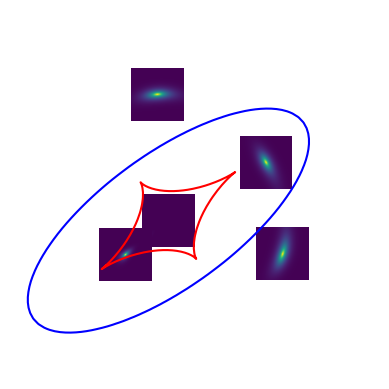
This is much more efficient than evaluating a whole image. Below you can see the same setup but we see how the simulator spends a lot of pixels evaluating low flux areas that don’t matter much for modelling.

sim_wide = caustics.LensSource(lens=lens, source=src, pixelscale=0.005, pixels_x=1000)
fig, ax = plt.subplots()
CS = ax.contour(thx, thy, detA, levels=[0.0], colors="b", zorder=1)
for path in paths:
    # Collect the path into a discrete set of points
    x1 = torch.tensor(list(float(vs[0]) for vs in path))
    x2 = torch.tensor(list(float(vs[1]) for vs in path))
    # raytrace the points to the source plane
    y1, y2 = lens.raytrace(x1, x2)

    # Plot the caustic
    ax.plot(y1, y2, color="r", zorder=1)
ax.imshow(
    sim_wide(),
    origin="lower",
    extent=(
        -sim_wide.pixelscale * sim_wide.pixels_x / 2,
        sim_wide.pixelscale * sim_wide.pixels_x / 2,
        -sim_wide.pixelscale * sim_wide.pixels_y / 2,
        sim_wide.pixelscale * sim_wide.pixels_y / 2,
    ),
)
ax.set_xlim([-1.5, 2])
ax.set_ylim([-1.5, 2])
ax.set_axis_off()
plt.show()

How forward_raytrace works

All forward raytracing methods are imperfect as they involve iterative solutions which require enough resolution to pick out all the relevant image plane positions. To start, lets consider a more naive algorithm, simply placing random points in the image plane, then running a root-finding algorithm to get the source plane positions to line up.

Ninit = 100
x_init = (torch.rand(Ninit) - 0.5) * fov
y_init = (torch.rand(Ninit) - 0.5) * fov


def raytrace(x, y):
    return lens.raytrace(x, y)


final = caustics.lenses.func.forward_raytrace_rootfind(
    x_init, y_init, sp_x, sp_y, raytrace
)
x_final, y_final = final[..., 0], final[..., 1]

# Pick only points that converged
bx_final, by_final = raytrace(x_final, y_final)
R = torch.sqrt((sp_x - bx_final) ** 2 + (sp_y - by_final) ** 2)
x_final = x_final[R < 1e-3]
x_init = x_init[R < 1e-3]
y_final = y_final[R < 1e-3]
y_init = y_init[R < 1e-3]

Here we easily find the four magnified images, but the central demagnified image is (often) not found by this method since a point has to get lucky enough to start very close to the correct position in order for the gradient based root finder to work.

Show code cell source

Hide code cell source

fig, ax = plt.subplots()
CS = ax.contour(thx, thy, detA, levels=[0.0], colors="b", zorder=1)
for path in paths:
    # Collect the path into a discrete set of points
    x1 = torch.tensor(list(float(vs[0]) for vs in path))
    x2 = torch.tensor(list(float(vs[1]) for vs in path))
    # raytrace the points to the source plane
    y1, y2 = lens.raytrace(x1, x2)

    # Plot the caustic
    ax.plot(y1, y2, color="r", zorder=1)
colors = ["tab:red", "tab:blue", "tab:green", "tab:orange", "tab:purple"]
for c in colors:
    if x_final.shape[0] == 0:
        break
    R = ((x_final[0] - x_final) ** 2 + (y_final[0] - y_final) ** 2).sqrt()
    ax.scatter(x_init[R < 0.1], y_init[R < 0.1], color=c)
    ax.scatter(x_final[0], y_final[0], color="k", s=200, marker="*")
    ax.scatter(x_final[0], y_final[0], color=c, s=100, marker="*")
    x_init = x_init[R >= 0.1]
    y_init = y_init[R >= 0.1]
    x_final = x_final[R >= 0.1]
    y_final = y_final[R >= 0.1]
ax.axes.set_axis_off()
ax.set_xlim([-fov / 1.9, fov / 1.9])
ax.set_ylim([-fov / 1.9, fov / 1.9])
plt.show()

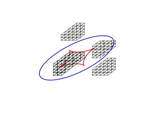
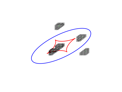
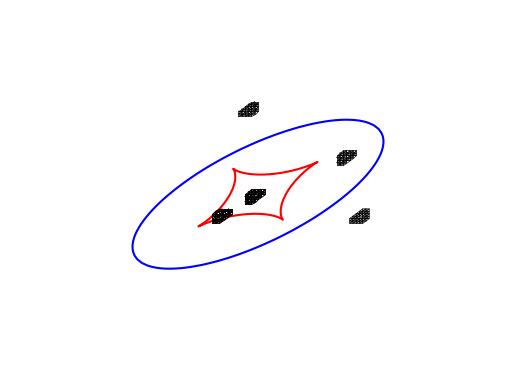
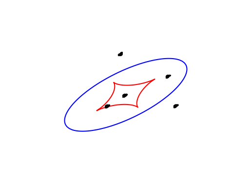
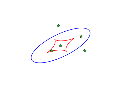
Let’s now look at a more clever algorithm. We will map triangles in the image plane to triangles in the source plane, we may then explore recursively, any triangles which enclose the desired source point. Due to the non-linearity of the gravitational lensing transformation, we will also search the neighbor of any triangle that seems to have found an image position. First we highlight in green, any triangles which contain the source point, then expand to all their neighbors.

Show code cell source

Hide code cell source

n = 10
s = torch.stack((sp_x, sp_y))
# Construct a tiling of the image plane (squares at this point)
X, Y = torch.meshgrid(
    torch.linspace(-fov / 2, fov / 2, n),
    torch.linspace(-fov / 2, fov / 2, n),
    indexing="ij",
)
E1 = torch.stack((X, Y), dim=-1)
# build the upper and lower triangles within the squares of the grid
E1 = torch.cat(
    (
        torch.stack((E1[:-1, :-1], E1[:-1, 1:], E1[1:, 1:]), dim=-2),
        torch.stack((E1[:-1, :-1], E1[1:, :-1], E1[1:, 1:]), dim=-2),
    ),
    dim=0,
).reshape(-1, 3, 2)
fig, ax = plt.subplots()
CS = ax.contour(thx, thy, detA, levels=[0.0], colors="b", zorder=1)
for path in paths:
    # Collect the path into a discrete set of points
    x1 = torch.tensor(list(float(vs[0]) for vs in path))
    x2 = torch.tensor(list(float(vs[1]) for vs in path))
    # raytrace the points to the source plane
    y1, y2 = lens.raytrace(x1, x2)

    # Plot the caustic
    ax.plot(y1, y2, color="r", zorder=1)
S = raytrace(E1[..., 0], E1[..., 1])
S = torch.stack(S, dim=-1)

# Identify triangles that contain the source plane point
locate1 = torch.vmap(caustics.lenses.func.triangle_contains, in_dims=(0, None))(S, s)
patches = []
for e, loc in zip(E1, locate1):
    patches.append(
        Polygon(
            e,
            fill=loc,
            alpha=0.4 if loc else 1,
            color="tab:green" if loc else "k",
            linewidth=1,
        )
    )
p = PatchCollection(patches, match_original=True)
ax.add_collection(p)
ax.set_xlim([-fov / 1.9, fov / 1.9])
ax.set_ylim([-fov / 1.9, fov / 1.9])
ax.set_axis_off()
plt.show()

# Get all the neighbors and upsample the triangles
E2 = E1[locate1]
E2 = torch.vmap(caustics.lenses.func.triangle_neighbors)(E2)
E2 = E2.reshape(-1, 3, 2)
E2 = caustics.lenses.func.remove_triangle_duplicates(E2)
# Upsample the triangles
E2 = torch.vmap(caustics.lenses.func.triangle_upsample)(E2)
E2 = E2.reshape(-1, 3, 2)

fig, ax = plt.subplots()
CS = ax.contour(thx, thy, detA, levels=[0.0], colors="b", zorder=1)
for path in paths:
    # Collect the path into a discrete set of points
    x1 = torch.tensor(list(float(vs[0]) for vs in path))
    x2 = torch.tensor(list(float(vs[1]) for vs in path))
    # raytrace the points to the source plane
    y1, y2 = lens.raytrace(x1, x2)

    # Plot the caustic
    ax.plot(y1, y2, color="r", zorder=1)
S = raytrace(E2[..., 0], E2[..., 1])
S = torch.stack(S, dim=-1)

# Identify triangles that contain the source plane point
locate2 = torch.vmap(caustics.lenses.func.triangle_contains, in_dims=(0, None))(S, s)
patches = []
for e, loc in zip(E2, locate2):
    patches.append(
        Polygon(
            e,
            fill=loc,
            alpha=0.4 if loc else 1,
            color="tab:green" if loc else "k",
            linewidth=0.5,
        )
    )
p = PatchCollection(patches, match_original=True)
ax.add_collection(p)
ax.set_xlim([-fov / 1.9, fov / 1.9])
ax.set_ylim([-fov / 1.9, fov / 1.9])
ax.set_axis_off()
plt.show()

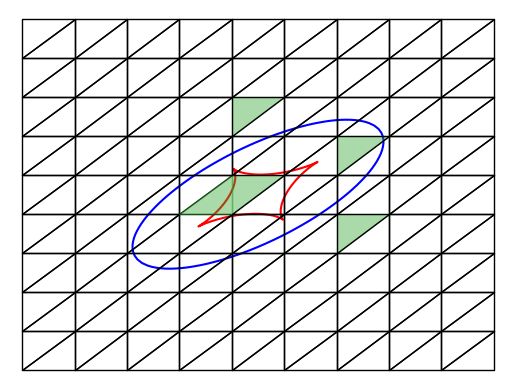
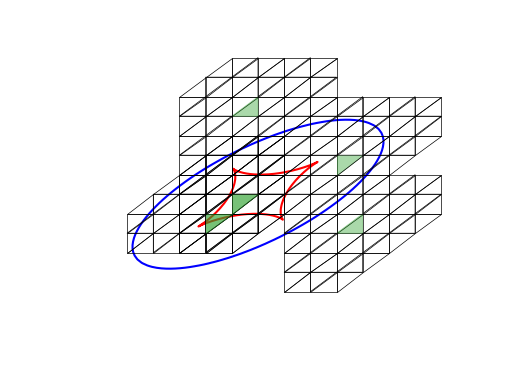
The process repeats until the triangles have converged to a very small area, at which point we then run a root finding algorithm to get the final points. The central region is a very unstable optimum, so we need to use the triangle method for several iterations before we can run the root finder to get the exact optimal point.

Show code cell source

Hide code cell source

# Get all the neighbors and upsample the triangles
E3 = E2[locate2]
E3 = torch.vmap(caustics.lenses.func.triangle_neighbors)(E3)
E3 = E3.reshape(-1, 3, 2)
E3 = caustics.lenses.func.remove_triangle_duplicates(E3)
# Upsample the triangles
E3 = torch.vmap(caustics.lenses.func.triangle_upsample)(E3)
E3 = E3.reshape(-1, 3, 2)

fig, ax = plt.subplots()
CS = ax.contour(thx, thy, detA, levels=[0.0], colors="b", zorder=1)
for path in paths:
    # Collect the path into a discrete set of points
    x1 = torch.tensor(list(float(vs[0]) for vs in path))
    x2 = torch.tensor(list(float(vs[1]) for vs in path))
    # raytrace the points to the source plane
    y1, y2 = lens.raytrace(x1, x2)

    # Plot the caustic
    ax.plot(y1, y2, color="r", zorder=1)
S = raytrace(E3[..., 0], E3[..., 1])
S = torch.stack(S, dim=-1)

# Identify triangles that contain the source plane point
locate3 = torch.vmap(caustics.lenses.func.triangle_contains, in_dims=(0, None))(S, s)
patches = []
for e, loc in zip(E3, locate3):
    patches.append(
        Polygon(
            e,
            fill=loc,
            alpha=0.4 if loc else 1,
            color="tab:green" if loc else "k",
            linewidth=0.5,
        )
    )
p = PatchCollection(patches, match_original=True)
ax.add_collection(p)
ax.set_xlim([-fov / 1.9, fov / 1.9])
ax.set_ylim([-fov / 1.9, fov / 1.9])
ax.set_axis_off()
plt.show()

# Get all the neighbors and upsample the triangles
E4 = E3[locate3]
E4 = torch.vmap(caustics.lenses.func.triangle_neighbors)(E4)
E4 = E4.reshape(-1, 3, 2)
E4 = caustics.lenses.func.remove_triangle_duplicates(E4)
# Upsample the triangles
E4 = torch.vmap(caustics.lenses.func.triangle_upsample)(E4)
E4 = E4.reshape(-1, 3, 2)

fig, ax = plt.subplots()
CS = ax.contour(thx, thy, detA, levels=[0.0], colors="b", zorder=1)
for path in paths:
    # Collect the path into a discrete set of points
    x1 = torch.tensor(list(float(vs[0]) for vs in path))
    x2 = torch.tensor(list(float(vs[1]) for vs in path))
    # raytrace the points to the source plane
    y1, y2 = lens.raytrace(x1, x2)

    # Plot the caustic
    ax.plot(y1, y2, color="r", zorder=1)
S = raytrace(E4[..., 0], E4[..., 1])
S = torch.stack(S, dim=-1)

# Identify triangles that contain the source plane point
locate4 = torch.vmap(caustics.lenses.func.triangle_contains, in_dims=(0, None))(S, s)
patches = []
for e, loc in zip(E4, locate4):
    patches.append(
        Polygon(
            e,
            fill=loc,
            alpha=0.4 if loc else 1,
            color="tab:green" if loc else "k",
            linewidth=0.5,
        )
    )
p = PatchCollection(patches, match_original=True)
ax.add_collection(p)
ax.set_xlim([-fov / 1.9, fov / 1.9])
ax.set_ylim([-fov / 1.9, fov / 1.9])
ax.set_axis_off()
plt.show()

# Get all the neighbors and upsample the triangles
E5 = E4[locate4]
E5 = torch.vmap(caustics.lenses.func.triangle_neighbors)(E5)
E5 = E5.reshape(-1, 3, 2)
E5 = caustics.lenses.func.remove_triangle_duplicates(E5)
# Upsample the triangles
E5 = torch.vmap(caustics.lenses.func.triangle_upsample)(E5)
E5 = E5.reshape(-1, 3, 2)

fig, ax = plt.subplots()
CS = ax.contour(thx, thy, detA, levels=[0.0], colors="b", zorder=1)
for path in paths:
    # Collect the path into a discrete set of points
    x1 = torch.tensor(list(float(vs[0]) for vs in path))
    x2 = torch.tensor(list(float(vs[1]) for vs in path))
    # raytrace the points to the source plane
    y1, y2 = lens.raytrace(x1, x2)

    # Plot the caustic
    ax.plot(y1, y2, color="r", zorder=1)
S = raytrace(E5[..., 0], E5[..., 1])
S = torch.stack(S, dim=-1)

# Identify triangles that contain the source plane point
locate5 = torch.vmap(caustics.lenses.func.triangle_contains, in_dims=(0, None))(S, s)

patches = []
for e, loc in zip(E5, locate5):
    patches.append(
        Polygon(
            e,
            fill=loc,
            alpha=0.4 if loc else 1,
            color="tab:green" if loc else "k",
            linewidth=0.5,
        )
    )
p = PatchCollection(patches, match_original=True)
ax.add_collection(p)
ax.set_xlim([-fov / 1.9, fov / 1.9])
ax.set_ylim([-fov / 1.9, fov / 1.9])
ax.set_axis_off()
plt.show()

# Get all the neighbors and upsample the triangles
E6 = E5[locate5]
E6 = torch.vmap(caustics.lenses.func.triangle_neighbors)(E6)
E6 = E6.reshape(-1, 3, 2)
E6 = caustics.lenses.func.remove_triangle_duplicates(E6)
# Upsample the triangles
E6 = torch.vmap(caustics.lenses.func.triangle_upsample)(E6)
E6 = E6.reshape(-1, 3, 2)

fig, ax = plt.subplots()
CS = ax.contour(thx, thy, detA, levels=[0.0], colors="b", zorder=1)
for path in paths:
    # Collect the path into a discrete set of points
    x1 = torch.tensor(list(float(vs[0]) for vs in path))
    x2 = torch.tensor(list(float(vs[1]) for vs in path))
    # raytrace the points to the source plane
    y1, y2 = lens.raytrace(x1, x2)

    # Plot the caustic
    ax.plot(y1, y2, color="r", zorder=1)
S = raytrace(E6[..., 0], E6[..., 1])
S = torch.stack(S, dim=-1)

# Identify triangles that contain the source plane point
locate6 = torch.vmap(caustics.lenses.func.triangle_contains, in_dims=(0, None))(S, s)

patches = []
for e, loc in zip(E6, locate6):
    patches.append(
        Polygon(
            e,
            fill=loc,
            alpha=0.4 if loc else 1,
            color="tab:green" if loc else "k",
            linewidth=0.5,
        )
    )
p = PatchCollection(patches, match_original=True)
ax.add_collection(p)
ax.set_xlim([-fov / 1.9, fov / 1.9])
ax.set_ylim([-fov / 1.9, fov / 1.9])
ax.set_axis_off()
plt.show()


# Run the root finding algorithm
E7 = E6[locate6].sum(dim=1) / 3
E7 = caustics.lenses.func.forward_raytrace_rootfind(
    E7[..., 0], E7[..., 1], s[0], s[1], raytrace
)
fig, ax = plt.subplots()
CS = ax.contour(thx, thy, detA, levels=[0.0], colors="b", zorder=1)
for path in paths:
    # Collect the path into a discrete set of points
    x1 = torch.tensor(list(float(vs[0]) for vs in path))
    x2 = torch.tensor(list(float(vs[1]) for vs in path))
    # raytrace the points to the source plane
    y1, y2 = lens.raytrace(x1, x2)

    # Plot the caustic
    ax.plot(y1, y2, color="r", zorder=1)
ax.scatter(E7[..., 0], E7[..., 1], color="k", s=100, marker="*")
ax.scatter(E7[..., 0], E7[..., 1], color="tab:green", s=50, marker="*")
ax.set_xlim([-fov / 1.9, fov / 1.9])
ax.set_ylim([-fov / 1.9, fov / 1.9])
ax.set_axis_off()
plt.show()